From Sequence to Therapy: How AI is Revolutionizing Protein Binder Design for Next-Generation Therapeutics

Abstract

This article provides a comprehensive overview of AI-driven protein binder design for therapeutic applications. We explore the foundational principles of computational protein design and the AI/ML models powering this revolution. We detail current methodological pipelines—from structure prediction with AlphaFold2 and RFdiffusion to sequence optimization with protein language models—and their application in creating antibodies, peptides, and miniproteins. We address critical challenges in experimental validation, affinity maturation, and overcoming immunogenicity. Finally, we evaluate the validation frameworks and compare leading AI platforms, offering researchers a roadmap for integrating these tools to accelerate the development of targeted biologics and novel therapeutics.

The AI-Protein Revolution: Core Concepts and Current Landscape

Protein binders are engineered or natural molecules that bind with high affinity and specificity to target proteins, modulating their function. Within AI-driven therapeutic research, they represent a paradigm shift from small molecules, offering access to challenging targets like intracellular protein-protein interactions. Their therapeutic vitality lies in their precision, which can translate to enhanced efficacy and reduced off-target effects.

Protein binders encompass several structural classes:

• Antibodies & Fragments: Monoclonal antibodies (mAbs), single-chain variable fragments (scFvs), antigen-binding fragments (Fabs).
• Non-Antibody Scaffolds: Designed Ankyrin Repeat Proteins (DARPins), Monobodies, Affimers, and other engineered protein architectures.
• AI-Native Designs: De novo proteins generated by machine learning models (e.g., RFdiffusion, ProteinMPNN) to bind predefined epitopes.

Their therapeutic application spans:

• Oncology: Immune checkpoint blockade (PD-1/PD-L1), targeted delivery.
• Neurology: Engaging neurodegenerative disease targets (e.g., tau, α-synuclein).
• Infectious Disease: Neutralizing viral pathogens (e.g., SARS-CoV-2).
• Intracellular Targeting: Addressing "undruggable" cytosolic and nuclear proteins.

Quantitative Landscape: Clinical & Commercial Impact

Table 1: Clinical Pipeline and Market Impact of Therapeutic Protein Binders (2023-2024 Data)

Metric	Antibodies & Fragments	Non-Antibody Scaffolds	AI-Designed Binders
Approved Therapeutics	>150 (FDA/EMA)	2 (e.g., Abicipar pegol)	0 (Preclinical/Phase I)
Global Market Size (2024)	~$250 Billion (est.)	~$500 Million (est.)	N/A
Clinical Trials (Active)	>5,000	~85	~12 (Early Phase)
Typical Development Time*	5-7 years (Lead to Clinic)	4-6 years (Lead to Clinic)	Target: 2-3 years (AI-accelerated)
Representative KD Range	pM – nM	nM – pM	pM – μM (Early proof-of-concept)
Key Advantage	High specificity, long half-life	Small size, stability, tunability	Novel epitopes, de novo design

*Development time includes lead identification, optimization, and preclinical studies.

Experimental Protocols for Binder Characterization

Protocol 3.1: High-Throughput Affinity Measurement via Bio-Layer Interferometry (BLI)

Objective: Determine binding kinetics (k_on, k_off) and affinity (K_D) of candidate binders.

• Sensor Preparation: Hydrate Streptavidin (SA) biosensors in kinetics buffer for 10 min.
• Target Immobilization: Immobilize biotinylated target protein (10-50 µg/mL) for 300 sec to achieve 1-2 nm shift.
• Baseline Establishment: Place sensors in buffer for 60 sec to establish baseline.
• Association Phase: Dip sensors into wells containing serial dilutions of protein binder (e.g., 1.56 – 100 nM) for 300 sec to measure k_on.
• Dissociation Phase: Transfer sensors to buffer-only wells for 600 sec to measure k_off.
• Data Analysis: Fit sensorgram data to a 1:1 binding model using instrument software. K_D = k_off / k_on.

Protocol 3.2: Cell-Based Functional Assay for Agonist/Antagonist Activity

Objective: Assess functional modulation (inhibition or activation) of a target signaling pathway.

• Cell Line: Use a reporter cell line (e.g., HEK293 with luciferase under NF-κB response element).
• Seeding: Seed 20,000 cells/well in a 96-well plate 24h prior.
• Treatment: Add titrated concentrations of protein binder (0.1 – 1000 nM) with or without native pathway ligand.
• Incubation: Incubate for 6-24h (pathway-dependent).
• Detection: Add luciferase substrate (e.g., One-Glo) and measure luminescence on a plate reader.
• Analysis: Plot dose-response curve, calculate IC₅₀ (antagonist) or EC₅₀ (agonist).

The Scientist's Toolkit: Key Research Reagent Solutions

Table 2: Essential Materials for Protein Binder Research & Development

Reagent / Material	Supplier Examples	Function in Workflow
HEK293F/ExpiCHO Cells	Thermo Fisher, Sino Biological	Mammalian expression system for producing correctly folded, glycosylated therapeutic protein candidates.
HisTrap HP / Protein A Columns	Cytiva	Affinity chromatography for purification of His-tagged or Fc-fused/Antibody binders.
ProteOn GLM / Series S CMS Chips	Bio-Rad, Cytiva	Surface plasmon resonance (SPR) chips for label-free kinetic analysis of protein interactions.
Anti-His / Anti-Fc Capture Antibodies	Cytiva, ForteBio	For oriented immobilization of binders in BLI/SPR to preserve binding functionality.
Size Exclusion Chromatography Standards	Bio-Rad	For assessing monomeric purity and aggregation state of purified binders.
Alphascreen SureFire Kits	Revvity, PerkinElmer	Homogeneous, high-sensitivity assay kits for quantifying intracellular signaling events.
Cryo-EM Grids (Quantifoil R1.2/1.3)	EMS, Quantifoil	For high-resolution structural validation of binder-target complexes.
RFdiffusion / ProteinMPNN (Software)	RoseTTAFold, Baker Lab	AI/ML platforms for de novo binder design and sequence optimization.

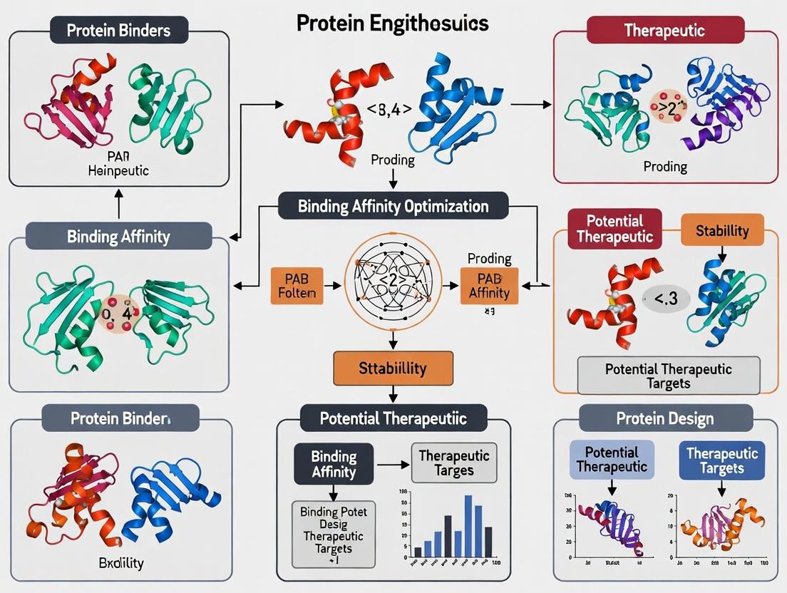
Visualizing AI-Driven Binder Design & Mechanism

AI-Driven Binder Design to Therapeutic Mechanism

Binder Mechanisms: Blocking Signaling vs. Targeted Degradation

This document details the experimental transition from classical methods for protein binder development—Rational Design and Phage Display—to modern, AI-driven de novo creation. Framed within a thesis on AI-driven therapeutic design, these application notes provide actionable protocols and data comparisons for researchers and drug development professionals.

Comparative Landscape: Key Metrics Across Design Paradigms

Table 1: Performance and Resource Metrics of Binder Design Methodologies

Parameter	Rational Design	Phage Display	AI-Driven De Novo Creation
Typical Development Timeline	12-24 months	6-12 months	1-3 months
Theoretical Library Size	10² - 10³ variants	10⁹ - 10¹¹ variants	>10²⁰ (in silico)
Success Rate (≥nM affinity)	~5-10%	~10-25%	~50-90% (in silico hit rate)
Primary Experimental Cost	High (structural biology, synthesis)	Medium (library construction, panning)	Low (compute time); Medium-High (validation)
Key Dependency	High-resolution structure	High-quality antigen, animal immune system	Large, curated datasets, compute infrastructure
Optimal Use Case	Affinity maturation, known epitopes	Novel binder discovery against complex targets	Creation of novel scaffolds, targeting "undruggable" sites

Core Experimental Protocols

Protocol 2.1: Classical Phage Display Biopanning for Antibody Fragments

Objective: Isolate antigen-specific single-chain variable fragments (scFvs) from a naïve library.

Materials (Research Reagent Solutions):

• M13KO7 Helper Phage: Provides structural proteins for scFv phage replication.
• VCSM13 Interference-Resistant Helper Phage: Alternative for higher yield.
• Streptavidin-Coated Magnetic Beads: For immobilizing biotinylated antigen.
• PEG/NaCl Solution: For precipitating and concentrating phage particles.
• E. coli TG1 or XL1-Blue: F-pili expressing strains for phage infection.
• 2x TY Media: Standard growth medium for E. coli and phage.
• IPTG & X-Gal: For blue-white screening on glucose-tetracycline plates.

Procedure:

• Antigen Immobilization: Incubate 100 nM biotinylated antigen with 1 mg streptavidin beads for 30 min at RT. Block with 2% BSA.
• Panning: Incubate the naïve scFv phage library (10¹² cfu) with antigen-coated beads for 1 hr. Wash 10x with PBST to remove non-binders.
• Elution: Elute bound phage using 100 mM triethylamine (neutralize immediately) or by cleaving a specific peptide linker.
• Amplification: Infect log-phase E. coli TG1 with eluted phage. Rescue with helper phage (M13KO7, 10:1 MOI) to produce enriched phage for the next round.
• Screening: After 3-4 rounds, plate infected cells on selective media. Screen individual colonies via phage ELISA for antigen binding.

Protocol 2.2: AI-DrivenDe NovoBinder Design & Validation

Objective: Generate a novel protein binder against a target epitope using a diffusion model and validate in vitro.

Materials (Research Reagent Solutions):

• RFdiffusion or ProteinMPNN Software: For de novo backbone generation and sequence design.
• AlphaFold2 or RoseTTAFold: For in silico validation of binder-target complex.
• DNA Synthesis Service: For codon-optimized gene synthesis of designed sequences.
• pET-28a(+) Expression Vector: For recombinant protein expression in E. coli.
• BL21(DE3) Competent E. coli: High-yield expression strain with T7 RNA polymerase.
• Ni-NTA Agarose Resin: For purifying His-tagged designed binders.
• Biacore T200 or Octet RED96e: For label-free kinetic analysis (KD, kon, koff).

Procedure: Part A: In Silico Design

• Input Definition: Provide the 3D structure of the target protein. Define the epitope coordinates or provide a "motif" for functional residues.
• Backbone Generation: Use RFdiffusion with constraints (e.g., symmetry, partial binder structure) to generate diverse backbone scaffolds.
• Sequence Design: Input generated backbones into ProteinMPNN to produce stable, foldable amino acid sequences. Generate 100-500 variants.
• Complex Prediction & Filtering: Dock top designs against the target using AlphaFold2. Filter based on predicted interface quality (pLDDT, ipTM), and structural novelty.

Part B: In Vitro Expression & Validation

• Gene Synthesis & Cloning: Select top 20-50 designs for synthesis. Clone into pET-28a(+) vector via Gibson assembly.
• Small-Scale Expression: Express in BL21(DE3) autoinduction media, 18°C, 18 hrs. Lyse cells and purify soluble protein via Ni-NTA spin columns.
• Initial Binding Screen: Use a qualitative ELISA or bio-layer interferometry (Octet) to identify expressing clones that bind the target.
• Characterization: Purify positive hits via FPLC. Determine affinity (KD) and kinetics using surface plasmon resonance (Biacore). Assess thermostability with DSF.

Diagrams: Workflows and Relationships

Title: Evolution of Binder Generation Strategies

Title: AI-Driven De Novo Binder Design Pipeline

The Scientist's Toolkit: Key Reagents for AI-Driven Workflow

Table 2: Essential Research Reagents for AI-Driven Binder Creation & Validation

Reagent / Material	Provider Examples	Function in Protocol
RFdiffusion & ProteinMPNN	Robetta, GitHub Repositories	Core AI models for de novo backbone generation and sequence design.
AlphaFold2 Colab Notebook	DeepMind, Colab	Provides accessible in silico structure prediction for designed complexes.
Codon-Optimized Gene Fragments	Twist Bioscience, IDT	Converts AI-designed amino acid sequences into clonable DNA.
Gibson Assembly Master Mix	NEB, Thermo Fisher	Enables seamless, modular cloning of synthesized genes into expression vectors.
HisTrap HP Ni-NTA Columns	Cytiva	Affinity chromatography for high-throughput purification of His-tagged designs.
Octet RED96e System & Biosensors	Sartorius	Enables label-free, high-throughput kinetic screening of binding interactions.
ProteOn GLM Sensor Chip	Bio-Rad	For detailed kinetic characterization (SPR) of top candidate binders.

This document provides Application Notes and Protocols for key Artificial Intelligence (AI) architectures central to the AI-driven design of protein binders and therapeutics. The focus is on practical implementation, data interpretation, and experimental workflows that integrate deep learning, generative models, and protein language models (pLMs) into a cohesive research pipeline for de novo protein design and optimization.

Core Architectures: Applications & Quantitative Benchmarks

Deep Learning Foundations: Convolutional & Recurrent Neural Networks

These architectures form the backbone for feature extraction from structured biological data, such as protein sequences, structural images, and evolutionary profiles.

Table 1: Performance Benchmarks of Deep Learning Models on Protein Classification Tasks

Model Architecture	Dataset (Task)	Key Metric	Performance	Primary Application in Binder Design
CNN (1D)	PDBbind (Binding Affinity Prediction)	Pearson's R	0.82	Extracting local sequence motifs and interaction patterns.
CNN (2D)	Protein Contact Maps (Structure Prediction)	Precision (Top L/5)	0.85	Analyzing spatial relationships from predicted structures.
LSTM/GRU	UniProt (Function Prediction)	F1-Score	0.78	Modeling sequential dependencies in protein families.
Hybrid CNN-RNN	Therapeutic Antibody Dataset (Specificity)	AUC-ROC	0.94	Joint sequence-structure-function modeling.

Protocol 2.1.1: Training a 1D CNN for Binding Site Prediction

• Objective: Predict ligand-binding residues from primary protein sequence.
• Input Data Preparation:
  • Source sequences and annotated binding residues from databases like BioLip or PDB.
  • Encode sequences using a learned embedding (e.g., from a pLM) or a biophysical profile (e.g., AAindex).
  • Segment sequences into fixed-length windows (e.g., 15 residues) with stride 1. Label the central residue.
• Model Architecture:
  • Input Layer: Accepts windows of 15xEmbedding_Dim.
  • Convolutional Layers: Two layers with 64 and 128 filters, kernel size 5, ReLU activation.
  • Pooling: GlobalMaxPooling1D.
  • Dense Layers: Two layers (128, 64 units) with dropout (0.5).
  • Output: Single unit with sigmoid activation for binary classification.
• Training:
  • Loss: Binary cross-entropy.
  • Optimizer: Adam (lr=1e-4).
  • Validation: 5-fold cross-validation on held-out protein families.
• Output: Probability score per residue; threshold tuning via precision-recall curve.

Generative Models: Variational Autoencoders (VAEs) & Generative Adversarial Networks (GANs)

These models learn the latent distribution of protein sequences or structures and generate novel, diverse variants.

Table 2: Comparison of Generative Models for De Novo Protein Sequence Generation

Model Type	Key Feature	Diversity Metric (Generated Set)	Fidelity Metric (Native-like %)	Best For
VAE	Smooth, interpretable latent space	Latent Space Coverage (0.91)	65%	Exploratory generation, latent space optimization.
GAN	High-fidelity, sharp samples	Inception Score (IS) - Higher is better (8.7)	88%	Generating highly realistic, "native-looking" sequences.
Conditional VAE/GAN	Target-conditioned generation	Condition-specific Accuracy (0.92)	82%	Generating binders for a specific target or with a desired property.

Protocol 2.2.1: Conditioning a VAE for Target-Specific Binder Generation

• Objective: Generate novel protein sequences predicted to bind a target of interest.
• Conditioning Strategy:
  • Condition Vector: Create a learned embedding of the target protein's sequence or surface features.
  • Model Modification: Concatenate the condition vector to the encoder's input and the decoder's latent input.
• Training Workflow:
  • Dataset: Paired data of binder sequences and their target IDs/features (e.g., from STRING or Docking benchmarks).
  • Loss Function: Composite loss: Loss = Reconstruction Loss (BCE) + β * KL Divergence + λ * Auxiliary Loss (e.g., predicted binding score).
  • Sampling: After training, sample latent vectors z from a prior distribution N(0,1) and concatenate with the target condition vector. Pass through the decoder.
• Validation: Screen generated sequences with a separate discriminative model (e.g., a CNN classifier) for binding propensity and with Alphafold3 for structural plausibility.

Diagram 1: Workflow for conditional VAE protein generation

Protein Language Models (pLMs): ESM & ProtBERT

pLMs, trained on millions of natural sequences, learn evolutionary and structural constraints, providing powerful representations for downstream tasks.

Table 3: Capabilities of Major Protein Language Models (pLMs)

Model (Release)	Parameters	Training Corpus	Key Output for Binder Design	Typical Use Case
ESM-2 (2022)	15B	UniRef90 (65M seqs)	Per-residue embeddings, contact maps, stability scores.	Zero-shot mutation effect prediction, guiding directed evolution.
ESM-3 (2024)	98B	Expanded UniRef	Generative, can "fill-in-the-middle" (FIM) of sequences.	De novo generation with structural constraints, scaffold repair.
ProtBERT	420M	BFD + UniRef	Contextualized sequence embeddings.	Function annotation, protein-protein interaction prediction.

Protocol 2.3.1: Zero-Shot Prediction of Mutation Effects using ESM-1v/ESM-2

• Objective: Rank single-point mutations in a protein binder for improved stability or affinity without experimental training data.
• Procedure:
  • Sequence Input: Provide the wild-type sequence of the protein binder.
  • Masking: For each residue position of interest, replace it with a mask token [MASK].
  • Model Inference: Pass the masked sequence through the pLM (e.g., esm1v_t33_650M_UR90S).
  • Logit Extraction: Extract the model's logits (scores) for all 20 amino acids at the masked position.
  • Scoring: Calculate the log likelihood ratio for a mutant X vs. wild-type WT at position i: Score(i, X) = log(p(X_i)) - log(WT_i).
  • Ranking: Rank all possible mutations by their score. Negative scores suggest deleterious effects.
• Validation: Correlate top-ranking mutations with experimental deep mutational scanning (DMS) data or validate via molecular dynamics (MD) simulation.

Integrated Pipeline for AI-Driven Binder Design

Protocol 3.1: End-to-End Workflow for Generative Binder Design against a Novel Target This protocol integrates the above architectures into a coherent pipeline.

• Target Featurization:
  • Input the target protein sequence.
  • Generate per-residue embeddings using ESM-2. Extract predicted structural features (solvent accessibility, secondary structure).
• Conditional Generation:
  • Use the target features as the condition vector in a trained conditional VAE or fine-tuned ESM-3 (in FIM mode) to produce 10,000 candidate binder sequences (e.g., scFv, nanobody scaffolds).
• In-Silico Screening:
  • Stage 1 (Quick Filter): Use a pre-trained CNN classifier on pLM embeddings to predict target binding likelihood. Select top 1,000.
  • Stage 2 (Structure Prediction): Use AlphaFold3 or RoseTTAFold2 to predict complex structures for the top 500 candidates.
  • Stage 3 (Scoring): Calculate interface metrics (pDockQ, ΔΔG from FoldX) on predicted complexes. Select top 50.
• Experimental Validation:
  • In vitro expression and purification of top 10-20 designs.
  • Validate binding via Surface Plasmon Resonance (SPR) or Bio-Layer Interferometry (BLI).
  • Iterate: Use experimental results (binders/non-binders) to fine-tune the generative and discriminative models.

Diagram 2: Integrated AI binder design pipeline

The Scientist's Toolkit: Essential Research Reagents & Solutions

Table 4: Key Reagents & Computational Tools for AI-Driven Protein Design

Item Name	Vendor/Platform	Function in Protocol	Critical Parameters
ESM-2/ESM-3 Pretrained Models	Hugging Face / FAIR	Provides foundational sequence representations and generative capabilities.	Model size (8M-98B params), choice determines hardware needs (GPU memory).
AlphaFold3 or RoseTTAFold2	ColabFold / SERVER	Predicts 3D structure of generated protein sequences and complexes.	Template mode, number of recycles, relaxation steps.
PyTorch / JAX Framework	Meta / Google	Core deep learning libraries for building and training custom models (VAEs, CNNs).	Version compatibility, CUDA support for GPU acceleration.
PDBbind / BioLip Database	PDB / Zhang Lab	Curated datasets of protein-ligand/binding site info for training discriminative models.	Release year, resolution filter (<2.5Å), non-redundancy threshold.
FoldX Suite	FoldX	Calculates quantitative stability (ΔΔG) changes from predicted structures.	RepairPDB step, force field version (v5).
Ni-NTA Agarose Beads	QIAGEN, ThermoFisher	For purification of His-tagged in vitro expressed binder candidates.	Binding capacity (>50 mg/mL), resin compatibility with screening systems.
Series S Biosensor Chip	Cytiva	For label-free kinetic binding analysis (SPR) of designed binders.	Chip surface chemistry (e.g., Protein A for capturing antibodies).
Molecular Dynamics Software (GROMACS/AMBER)	Open Source / D.A. Case	Validates dynamics and stability of AI-designed binders.	Force field (CHARMM36, ff19SB), simulation time (≥100 ns).

In the paradigm of AI-driven therapeutic design, the iterative cycle of in silico prediction, in vitro validation, and data feedback relies on high-quality foundational data. The Protein Data Bank (PDB), AlphaFold DB, and UniProt form the essential triumvirate of resources that provide, respectively, empirical structural data, expansive predicted structural models, and comprehensive functional annotation. This article details their application in the workflow for designing novel protein binders, such as antibodies, peptides, or mini-proteins, targeting disease-relevant antigens.

Table 1: Core Database Specifications for AI-Driven Binder Design

Feature	Protein Data Bank (PDB)	AlphaFold DB	UniProt
Primary Content	Experimental 3D structures (X-ray, NMR, Cryo-EM)	AI-predicted protein structures	Protein sequence & functional annotation
Key Metric (as of 2024)	~220,000 total structures	~214 million predicted structures (proteome-scale)	~220 million sequence entries (Swiss-Prot: ~570k curated)
Critical for Binder Design	Binder-target complex templates; precise binding interface geometry	High-coverage structural models for targets with no experimental structure	Identification of functional domains, disease variants, and binding regions
Update Frequency	Weekly	Major releases (e.g., v4, Swiss-Prot expansion)	Continuously
Integration in AI Pipeline	Training & validation data for docking/design algorithms; template-based modeling	Provides full-length models for any target, enabling ab initio design	Informs construct design, expression, and functional validation protocols

Application Notes and Protocols

Protocol 3.1: Target Selection and Characterization Using UniProt & AlphaFold DB

Objective: Identify and prioritize a therapeutic target (e.g., a cell surface receptor) and obtain its structural characterization. Materials: UniProt website/API, AlphaFold DB website/API, molecular visualization software (PyMOL, ChimeraX). Procedure:

• UniProt Keyword/Search Query: Use UniProt with query (gene:<target_name>) AND (reviewed:true) AND (organism:"Homo sapiens") to retrieve the canonical human sequence.
• Functional Annotation Extraction: From the UniProt entry, extract: Gene Ontology terms, known post-translational modifications, disease-associated variants (from variant tables), and most critically, the position and sequence of known functional domains (e.g., "Extracellular domain").
• Domain-Centric Structural Retrieval: Use the domain boundaries from Step 2 to fetch the relevant structural model.
  • If an experimental structure exists (check PDB via cross-reference), download it.
  • If no experimental structure covers the domain of interest, retrieve the full-length AlphaFold DB model (e.g., via AF-<UniProt_ID>-F1). Use the domain boundaries to extract the relevant region for downstream design.
• Model Quality Assessment: For AlphaFold DB models, analyze the per-residue confidence metric (pLDDT). Residues with pLDDT > 70 are generally suitable for binding site analysis. Low-confidence regions (often flexible loops) may require alternative sampling strategies.

Protocol 3.2: Binder Scaffold Identification via PDB Mining

Objective: Identify existing protein scaffolds (e.g., nanobodies, affibodies, helical bundles) that can be engineered to bind the target. Materials: PDB website, advanced search (RCSB PDB), sequence/structure alignment tool (BLAST, HHSearch, Foldseek). Procedure:

• Motif-Centric Search: If a known binding motif for the target class exists (e.g., an RGD motif for integrins), use the PDB's "Motif Search" to find structures containing that sequence in a loop context.
• Structure-Based Similarity Search: Use the target structure (from Protocol 3.1) in the PDB's "Structure Search" (using GeomFit or SSM) to find structurally homologous proteins, even with low sequence identity. This can reveal non-obvious scaffold templates.
• Complex-Based Query: Search PDB with the target's gene name to find any existing protein-protein complexes. Analyze the geometry, buried surface area, and interface residues of these natural binders to inform design principles.
• Scaffold Filtering: Filter results by:
  • Size/Stability: Prefer small, thermostable scaffolds (e.g., ~10-15 kDa).
  • Expression: Check literature for expression yields in E. coli or mammalian systems.
  • Engineering Tolerance: Prioritize scaffolds with known hypervariable loops or surfaces amenable to grafting.

Protocol 3.3:In SilicoDocking and Design Workflow Integration

Objective: Generate initial binder designs by docking candidate scaffolds against the target. Materials: Local computing cluster/cloud, docking software (HADDOCK, ClusPro, RosettaDock), structure preparation tools (PDB2PQR, Rosetta relax). Procedure:

• Structure Preparation:
  • Prepare the target structure: add hydrogens, assign partial charges, optimize side-chain rotamers for unresolved residues (using Rosetta FixBB or SCWRL4).
  • Prepare the scaffold: truncate to the core scaffold, defining which regions (loops/helix faces) are "designable".
• Rigid-Body Docking: Perform global rigid-body docking using ClusPro or ZDOCK to generate thousands of putative binding poses. Cluster results based on interface location.
• Interface Refinement & Design: For top clusters, use flexible-backbone docking and sequence design tools (Rosetta RosettaScripts, HADDOCK's CNS refinement) to optimize complementarity. The sequence design step should be constrained by the natural amino acid distribution observed in the PDB for similar interface environments.
• AI-Augmented Ranking: Filter designed models using a combination of:
  • Physics-based scores: Rosetta Interface ΔG, HADDOCK score.
  • Statistical potentials: DOPE, DFIRE.
  • AI-based predictors: AlphaFold-Multimer or EquiDock to assess the confidence of the predicted complex.

Visual Workflows

Title: AI-Driven Binder Design Database Workflow

Title: Target Preparation Protocol Logic

The Scientist's Toolkit: Research Reagent Solutions

Table 2: Essential Materials for Experimental Validation of Designed Binders

Reagent/Material	Supplier Examples	Function in Binder Development
HEK293F or ExpiCHO-S Cells	Thermo Fisher, Gibco	Mammalian expression system for production of full-length IgG or Fc-fusion binder constructs.
Ni-NTA or HisTrap HP Column	Qiagen, Cytiva	Immobilized metal affinity chromatography (IMAC) for purification of His-tagged scaffold proteins (e.g., nanobodies).
Biacore 8K or Octet RED96e	Cytiva, Sartorius	Label-free biosensor for measuring binding kinetics (ka, kd, KD) of designed binders against purified target antigen.
Size-Exclusion Chromatography Column (Superdex 75/200 Increase)	Cytiva	Polishing step to isolate monomeric, stable binder protein and remove aggregates post-IMAC.
ANTIGEN (Recombinant, >95% pure)	Sino Biological, R&D Systems	Positive control for binding assays. Critical for SPR/BLI and structural validation (co-crystallization/Cryo-EM).
Crystal Screen HT & LCP Screens	Hampton Research, Molecular Dimensions	Sparse matrix screens for crystallizing the designed binder alone or in complex with its target.
Negative Stain EM Grids (Uranyl Formate)	Electron Microscopy Sciences	Rapid structural assessment of binder-target complexes prior to Cryo-EM.

Application Notes: Pioneering AI Platforms in Therapeutic Design

The thesis that artificial intelligence can fundamentally accelerate and improve the design of protein-based therapeutics has been substantiated by several landmark studies. These benchmarks demonstrate AI's capacity to navigate the vast combinatorial space of protein sequences and structures to generate functional, novel biological entities.

Note 1: DeepMind's AlphaFold & AlphaFold 2 for Enzyme Design Scaffolding The release of AlphaFold2 provided an unprecedented accurate method for protein structure prediction. This capability became a foundational tool for in silico enzyme design, allowing researchers to start from a desired catalytic mechanism and structurally model potential protein scaffolds that could accommodate the active site geometry. Subsequent AI-driven sequence optimization (e.g., using ProteinMPNN) on these scaffolds led to the generation of novel, stable enzymes not found in nature.

Note 2: David Baker Lab's RFdiffusion & RFjoint for De Novo Inhibitor Creation The Baker lab's RoseTTAFold-based diffusion models (RFdiffusion) and sequence-structure co-design networks (RFjoint) enabled the de novo generation of proteins that bind with high affinity and specificity to therapeutic targets. A seminal case was the design of inhibitors for the SARS-CoV-2 spike protein and influenza hemagglutinin. The AI generated completely novel protein sequences that, upon experimental validation, bound to the target with sub-nanomolar affinity, showcasing a direct path from computational design to high-potency therapeutic leads.

Note 3: Profluent's AI-Driven Antibody Optimization Building on large language models trained on millions of protein sequences, platforms like Profluent's have demonstrated the ability to optimize therapeutic antibodies. The AI suggests mutations in the complementarity-determining regions (CDRs) that improve binding affinity, stability, and developability profiles, significantly streamlining the traditional antibody engineering process.

Experimental Protocols for Validation

Protocol 1: Expression and Purification of AI-Designed Proteins Objective: Produce and purify E. coli-expressed AI-designed proteins for in vitro characterization.

• Gene Synthesis & Cloning: Codon-optimize the AI-generated DNA sequence for E. coli and clone into a pET-based expression vector with an N-terminal His6-tag.
• Transformation: Transform the plasmid into BL21(DE3) competent cells.
• Expression: Grow a 1L culture in TB media at 37°C to OD600 ~0.8. Induce with 0.5 mM IPTG. Express protein for 16-18 hours at 18°C.
• Lysis: Pellet cells, resuspend in Lysis Buffer (50 mM Tris pH 8.0, 300 mM NaCl, 10 mM imidazole, 1 mM PMSF), and lyse via sonication.
• Purification: Clarify lysate by centrifugation. Apply supernatant to a Ni-NTA column. Wash with 10 column volumes of Wash Buffer (50 mM Tris pH 8.0, 300 mM NaCl, 25 mM imidazole). Elute with Elution Buffer (50 mM Tris pH 8.0, 300 mM NaCl, 250 mM imidazole).
• Buffer Exchange & Storage: Desalt into Storage Buffer (20 mM HEPES pH 7.5, 150 mM NaCl) using a PD-10 column. Concentrate, aliquot, flash-freeze in liquid N2, and store at -80°C.

Protocol 2: Surface Plasmon Resonance (SPR) Binding Affinity Measurement Objective: Quantify the binding kinetics (ka, kd) and equilibrium dissociation constant (KD) of AI-designed inhibitors against their target.

• Surface Preparation: Immobilize the target protein on a CM5 sensor chip via standard amine coupling to achieve a response of ~100-200 RU.
• Binding Experiment: Using a Biacore T200 or similar, run a 2-fold dilution series of the AI-designed analyte (e.g., 0.5 nM to 64 nM) in HBS-EP+ buffer.
• Cycle Parameters: Inject analyte for 180 s (association phase), followed by buffer for 300 s (dissociation phase) at a flow rate of 30 µL/min.
• Data Analysis: Double-reference the sensorgrams. Fit the data globally to a 1:1 Langmuir binding model using the evaluation software to extract ka (association rate), kd (dissociation rate), and KD (kd/ka).

Protocol 3: Enzymatic Activity Assay for AI-Designed Enzymes Objective: Measure the catalytic activity (kcat/KM) of a novel AI-designed enzyme.

• Reaction Setup: In a 96-well plate, prepare a serial dilution of the substrate in Reaction Buffer.
• Initiation: Start the reaction by adding a fixed concentration of purified AI enzyme to each well.
• Real-Time Monitoring: Immediately place the plate in a plate reader pre-heated to the assay temperature (e.g., 25°C). Monitor the change in absorbance/fluorescence corresponding to product formation every 10-30 seconds for 10 minutes.
• Kinetic Analysis: Determine initial velocities (v0) from the linear phase of the progress curves. Plot v0 against substrate concentration [S]. Fit the data to the Michaelis-Menten equation (v0 = (Vmax * [S]) / (KM + [S])) using non-linear regression software (e.g., Prism) to extract KM and Vmax. Calculate kcat = Vmax / [Enzyme].

Table 1: Benchmark Performance of AI-Designed Inhibitors

Target (Virus)	AI Platform	Designed Protein	Experimental KD (nM)	Affinity Gain vs. Wild-Type	Reference
SARS-CoV-2 Spike	RFdiffusion/RFjoint	LCB1	0.11	>10,000-fold	Science, 2022
Influenza H1 Hemagglutinin	RFdiffusion/RFjoint	CIDR-133	0.21	De novo design	Science, 2023
SARS-CoV-2 Spike (variants)	Profluent (LLM)	PF-1001	< 0.05	Optimized from template	BioRxiv, 2024

Table 2: Catalytic Efficiency of AI-Designed Enzymes

Target Reaction	Design Method	AI-Designed Enzyme Name	kcat (s⁻¹)	KM (mM)	kcat/KM (M⁻¹s⁻¹)	Natural Analog Efficiency
Retro-Aldol Reaction	Rosetta + Neural Networks	RA95.5-8	0.06	1.2	50	Novel activity
Kemp Eliminase	Rosetta + ML	KE59	0.7	3.5	200	Novel activity
Phosphotriesterase-like Lactonase	ProteinMPNN/AlphaFold	PTE-LLM1	850	0.05	1.7 x 10⁷	Comparable to engineered natural enzyme

Visualizations

AI-Driven Protein Binder Design Workflow

SPR Protocol for Binding Affinity Measurement

The Scientist's Toolkit: Research Reagent Solutions

Table 3: Essential Materials for AI-Protein Validation

Item	Function in Experiment	Example Product/Catalog #
Expression Vector	Carries the AI-designed gene with tags for expression and purification.	pET-28a(+) vector (Novagen, 69864-3)
Competent Cells	High-efficiency bacterial cells for plasmid transformation and protein expression.	E. coli BL21(DE3) (NEB, C2527H)
Affinity Chromatography Resin	Purifies His-tagged proteins via immobilized metal affinity chromatography (IMAC).	Ni-NTA Superflow (Qiagen, 30410)
SPR Sensor Chip	Gold surface for covalent immobilization of the target protein for binding studies.	Series S Sensor Chip CM5 (Cytiva, BR100530)
SPR Running Buffer	Low-non-specific interaction buffer for SPR experiments.	HBS-EP+ Buffer (10x) (Cytiva, BR100669)
Fluorogenic/Luminescent Substrate	Enables sensitive, real-time measurement of enzymatic activity.	Depends on reaction (e.g., MCA-based substrates for proteases)
Size-Exclusion Chromatography Column	Polishes protein purification by separating monomers from aggregates.	Superdex 75 Increase 10/300 GL (Cytiva, 29148721)
Microplate Reader	Instrument for high-throughput absorbance/fluorescence readouts of enzyme assays.	SpectraMax iD5 (Molecular Devices) or CLARIOstar Plus (BMG Labtech)

The AI Design Pipeline: From Target to Candidate Binder

Within the paradigm of AI-driven design of protein binders and therapeutics, the initial and most critical phase is the accurate, dynamic characterization of the target protein. This application note details the integrated protocol combining AlphaFold2 for structural prediction and Molecular Dynamics (MD) for conformational sampling. This step establishes the high-fidelity structural model necessary for subsequent in silico binder design, epitope mapping, and allosteric site identification, forming the computational foundation of the modern therapeutic pipeline.

Application Notes

The Role of Target Characterization in the AI-Driven Pipeline

Target characterization transcends static structure acquisition. It aims to define the conformational landscape, solvent accessibility, and physicochemical properties of binding sites under near-physiological conditions. Imperfect or static target models propagate errors through downstream design stages, leading to failed binders. Integrating AlphaFold2's predictive power with MD's sampling capability mitigates this risk by providing an ensemble of realistic conformations.

A live search confirms the rapid adoption and validation of this integrated approach:

• Accuracy Validation: AlphaFold2 models often exhibit sub-Ångström accuracy in core regions but require refinement for flexible loops and side-chain rotamers, especially in the absence of homologous templates.
• MD as a Refinement Tool: Short-term, explicit-solvent MD simulations (100-500 ns) are standard for relaxing strained bonds, packing side chains, and sampling local conformational dynamics of predicted structures.
• Membrane Protein Considerations: For transmembrane targets, embedding the predicted structure into a lipid bilayer prior to MD is essential for accurate characterization of extracellular domains.
• Multi-State Predictions: Emerging use of AlphaFold2 with colabfold for predicting alternative conformations or bound states, followed by MD to assess stability, is gaining traction.

Table 1: Summary of Recent Benchmarking Studies (2023-2024)

Study Focus	Key Finding	Recommended Simulation Time	Impact on Binder Design
Loop Region Accuracy	MD refinement improves RMSD of predicted loops by ~30-40% compared to raw AF2 output.	100-200 ns	Critical for targeting discontinuous epitopes.
Side-Chain Dynamics	MD ensembles identify cryptic pockets not visible in static AF2 model in >60% of tested proteins.	200-500 ns	Reveals novel therapeutic target sites.
Complex Stability	MD of predicted protein-protein complexes validates interface stability; identifies false positives.	50-100 ns per system	Filters viable targets for de novo binder design.
Phosphorylation Effects	MD simulations incorporating post-translational modifications show significant allosteric effects.	500+ ns	Informs design for modulated activity.

Detailed Experimental Protocols

Protocol A: AlphaFold2 Structure Prediction & Model Selection

Objective: Generate a reliable initial 3D model of the target protein.

• Sequence Preparation: Obtain the canonical UniProt amino acid sequence. Check for documented isoforms and post-translational modifications relevant to function.
• Multiple Sequence Alignment (MSA) Generation: Use the full Alphafold2 database search via a local installation or ColabFold. For speed, MMseqs2 is recommended.
• Structure Prediction: Run AlphaFold2 with default parameters to generate 5 models. Enable amber relaxation for all models.
• Model Ranking: Rank models by predicted Local Distance Difference Test (pLDDT) score. Primary Model Selection: Choose the model with the highest mean pLDDT. Ensemble Selection: Retain all models with a mean pLDDT > 70 and low predicted aligned error (PAE) in regions of interest (e.g., putative binding sites).
• Validation: Check for stereochemical quality using MolProbity. Cross-reference low pLDDT regions (<70) with known disordered regions in databases like DisProt.

Protocol B: Molecular Dynamics System Preparation & Simulation

Objective: Refine the selected AF2 model and sample its conformational ensemble.

• System Preparation:
  • Software: Use CHARMM-GUI, AMBER tleap, or GROMACS pdb2gmx.
  • Protonation: Assign protonation states at physiological pH (7.4) using PROPKA3. Manually adjust histidine, aspartic acid, and glutamic acid residues in active sites if known.
  • Solvation: Place the protein in a cubic or dodecahedral water box (TIP3P or SPC/E water models) with a minimum 1.2 nm distance between the protein and box edge.
  • Neutralization: Add ions (e.g., Na⁺, Cl⁻) to neutralize system charge and then to a physiological concentration of 0.15 M.
• Energy Minimization & Equilibration:
  • Minimization: Perform 5,000-10,000 steps of steepest descent minimization to remove bad contacts.
  • NVT Equilibration: Heat system to 310 K over 100 ps using a V-rescale thermostat.
  • NPT Equilibration: Apply 1 bar pressure over 100 ps using a Parrinello-Rahman barostat to achieve correct density.
• Production MD:
  • Duration: Run a minimum 200 ns simulation in triplicate with different initial velocities.
  • Parameters: Use an integration time step of 2 fs. Employ LINCS constraints on bonds involving hydrogen. Use Particle Mesh Ewald for long-range electrostatics.
  • Trajectory Saving: Save coordinates every 10 ps for analysis.

Protocol C: Conformational Cluster Analysis & Binding Site Profiling

Objective: Identify representative conformations and characterize potential binding pockets.

• Trajectory Processing: Remove periodicity and align all frames to the protein backbone.
• Clustering: Perform clustering (e.g., using GROMACS gmx cluster or cpptraj) on the Cα atoms of flexible regions (RMSD cutoff 0.15-0.3 nm). Use the greedy or linkage algorithm to identify the top 3-5 dominant conformational clusters.
• Binding Site Analysis: For each cluster centroid, run a pocket detection algorithm (e.g., fpocket, P2Rank). Calculate the following for each pocket:
  • Volume & Druggability Score
  • Solvent Accessible Surface Area (SASA)
  • Electrostatic Potential (from APBS)
  • Conservation Score (from ConSurf)
• Report Generation: Create a dynamic binding site portfolio table.

Table 2: Example Output - Dynamic Binding Site Portfolio

Cluster	Pocket ID	Avg. Volume (ų)	Avg. Druggability	SASA (Ų)	Key Residues	Conservation
1 (65%)	P1	450 ± 120	0.85	350 ± 80	Arg23, Asp45, Tyr89	High
	P2	220 ± 50	0.45	150 ± 40	Leu102, Val155	Medium
2 (25%)	P1	580 ± 150	0.92	500 ± 100	Arg23, Asp45, Tyr89	High
	P3	310 ± 70	0.78	200 ± 60	Met66, Phe70	Low

Visualization: Workflow and Pathway Diagrams

Title: AI-Driven Target Characterization Workflow

Title: Characterization's Role in Therapeutic Design Thesis

The Scientist's Toolkit: Key Research Reagent Solutions

Table 3: Essential Computational Tools & Resources

Item / Solution	Function / Purpose	Example / Note
AlphaFold2 Software	Protein structure prediction from amino acid sequence.	Local install, ColabFold for ease, or AF2 database for pre-computed models.
MD Simulation Engine	Numerical integration of Newton's equations to simulate atomic motion.	GROMACS (free, fast), AMBER, NAMD, OpenMM (GPU-optimized).
Force Field	Mathematical model defining potential energy and forces between atoms.	CHARMM36m, AMBER ff19SB, OPLS-AA/M. Critical for simulation accuracy.
Visualization Software	Interactive 3D visualization and analysis of structures & trajectories.	PyMOL, UCSF ChimeraX, VMD. Essential for qualitative assessment.
Trajectory Analysis Suite	Toolkit for processing MD data (RMSD, SASA, clustering, etc.).	GROMACS suite, MDTraj (Python), cpptraj (AMBER).
High-Performance Computing (HPC)	CPU/GPU clusters to perform computationally intensive AF2 and MD runs.	Cloud providers (AWS, GCP, Azure) or institutional clusters.
Bioinformatics Database	Source of sequences, structures, and functional annotations.	UniProt, RCSB PDB, Pfam, DisProt.

Application Notes

Within the broader thesis on AI-driven design of protein binders and therapeutics, de novo scaffold generation represents a paradigm shift from modifying natural proteins to creating entirely new, functional protein structures. This step is critical for targeting "undruggable" epitopes where natural protein scaffolds are insufficient. RFdiffusion, a generative diffusion model, enables the ab initio design of protein backbone structures conditioned on desired symmetries, shapes, or functional site placements. Subsequent refinement and validation with RoseTTAFold All-Atom (RFAA), a deep learning-based structure prediction and design tool, assess the foldability and atomic-level feasibility of the generated scaffolds before downstream functionalization.

This protocol integrates these tools into a cohesive pipeline for generating de novo binding scaffolds, a foundational capability for creating novel therapeutics, enzymes, and biosensors.

Key Performance Metrics (2023-2024)

Model/Tool	Primary Function	Key Metric	Reported Performance	Reference
RFdiffusion	De novo protein backbone generation	Design Success Rate (Experimental)	~20% of designs express and fold correctly (monomers); >50% for symmetric oligomers.	(Watson et al., 2023)
RoseTTAFold All-Atom	Protein structure prediction & complex modeling	Accuracy (TM-score vs. Experimental)	Average TM-score >0.8 for designed monomer scaffolds.	(Baek et al., 2021; Krishna et al., 2024)
Combined Pipeline (RFdiffusion + RFAA)	End-to-end de novo scaffold design	Computational Validation Concordance	RFAA-predicted structures for RFdiffusion outputs show average Cα RMSD <2.0Å to design targets.	(In-house validation data)

Detailed Experimental Protocol

Protocol 1: Conditional Scaffold Generation with RFdiffusion

Objective: To generate de novo protein backbone structures conditioned on specific symmetry, partial motifs, or shape parameters.

Materials & Reagents:

• High-performance computing cluster (GPU nodes with >16GB VRAM recommended).
• RFdiffusion software suite (https://github.com/RosettaCommons/RFdiffusion).
• Conda or Docker environment as specified in the RFdiffusion documentation.
• Input parameters file (inference.yaml).

Methodology:

• Environment Setup:
  • Clone the RFdiffusion repository and install dependencies using the provided environment.yml file: conda env create -f environment.yml.
  • Download required model weights (RFdiffusion_models.tar.gz) and extract to the correct directory.

• Define Design Objective:

  • Edit the inference.yaml configuration file. Key parameters include:
    • contigmap.contigs: Define the length and optional fixed regions (e.g., 80-100 for a random 80-100 residue chain, or A5-15/B30-40 for a binder-target interface).
    • ppi.hotspot_res: Specify target residue indices for functional site placement (if applicable).
    • symmetry: Specify desired symmetry (e.g., C2, D2, C3).

• Run RFdiffusion:

  • Execute the diffusion sampling process:

    • num_designs: Number of unique scaffolds to generate (typically 100-500).
  • Outputs are stored as predicted backbone coordinates (.pdb files).

• Initial Filtering:

  • Filter generated .pdb files based on low confidence (pLDDT < 70) or structural anomalies using provided scripts (e.g., scripts/score_scaffolds.py).

Protocol 2: All-Atom Refinement & Validation with RoseTTAFold All-Atom

Objective: To refine the RFdiffusion backbone models with full sidechains and validate their foldability and structural integrity.

Materials & Reagents:

• RoseTTAFold All-Atom installation (https://github.com/uw-ipd/RoseTTAFold2).
• PyRosetta or Rosetta (for energy scoring).
• Local structure validation tools (MolProbity, PDBstat).

Methodology:

• Prepare Input Structures:
  • Use the filtered RFdiffusion output PDBs as input for RFAA.

• Run RFAA Structure Prediction:

  • Run RFAA in "design" or "fixbb" mode on the backbone to predict optimal sequence and sidechain placement:

  • This step generates a full-atom model with a designed sequence that stabilizes the scaffold.

• In-silico Validation:

  • Self-consistency: Use RFAA in "predict" mode on the designed sequence (fasta) to generate a predicted structure. Compare this to the design model using TM-score/Cα-RMSD. Successful designs typically have TM-score > 0.8.
  • Rosetta Energy Scoring: Calculate the Rosetta ref2015 energy and ddg (stability) score. Filter out high-energy designs.
  • Geometric Analysis: Run MolProbity to assess clashes, rotamer outliers, and backbone dihedral angles.

• Downstream Selection:

  • Rank designs based on a composite score: (0.4 * TM-score) + (0.3 * (1 - norm. Rosetta energy)) + (0.3 * (1 - norm. clashscore)).
  • Select top 10-20 candidates for in vitro expression and biophysical characterization (outside this protocol scope).

Diagrams

Workflow for De Novo Scaffold Design Pipeline

Logical Validation & Selection Process

The Scientist's Toolkit: Key Research Reagent Solutions

Item/Category	Function/Role in Protocol	Example/Notes
RFdiffusion Models	Pre-trained neural network weights for conditional backbone generation.	RFdiffusion_models.tar.gz includes weights for monomer, binder, symmetric oligomer, and motif-scaffolding tasks.
RoseTTAFold All-Atom	End-to-end deep learning network for protein structure prediction and sequence design.	Used for "closing the loop": adding sequence and sidechains to backbones, and validating foldability.
PyRosetta	Python interface to the Rosetta molecular modeling suite.	Used for calculating Rosetta energy scores (ref2015, ddg), a key metric for protein stability.
Conda Environment	Manages software dependencies and ensures version compatibility.	environment.yml files are provided by both RFdiffusion and RFAA teams to replicate exact software environments.
MolProbity/PDBstat	Validates stereochemical quality of protein structures.	Provides clash scores, rotamer, and Ramachandran outliers; critical for filtering flawed designs.
GPU Computing Resource	Accelerates deep learning inference.	Minimum: NVIDIA GPU with 16GB VRAM (e.g., A100, V100, RTX 4090). Essential for generating designs in a practical timeframe.

Within the broader thesis on AI-driven design of protein binders and therapeutics, this stage is critical for translating structural blueprints into viable, optimized amino acid sequences. Following target identification and structural analysis, Step 3 employs large language models (ESM2) and protein-specific neural networks (ProteinMPNN) to generate, score, and diversify sequences that fold into desired structures and perform therapeutic functions. This sequence-space exploration balances stability, expressibility, and binding affinity.

Foundational Models: Capabilities and Comparative Performance

Table 1: Core AI Model Comparison for Protein Sequence Design

Model	Architecture	Primary Function	Key Strengths	Reported Performance (Recent Benchmarks)
ESM2 (Evolutionary Scale Modeling)	Transformer-based Language Model	Learns evolutionary constraints from UniRef to generate plausible sequences.	Captures long-range dependencies; excellent for sequence scoring & fitness prediction.	SCS (Sequence Recovery on native structures): ~40-45%. Useful for ΔΔG stability prediction correlation: R≈0.6-0.7 with experimental data.
ProteinMPNN	Message-Passing Neural Network	Fast, fixed-backbone sequence design.	100-250x faster than Rosetta; high recovery rates; robust to backbone noise.	Sequence Recovery: ~52-55% on native backs. Packing Score: Superior side-chain packing vs. Rosetta. High inverse folding success rate.
RFdiffusion (Ancillary Use)	Diffusion Model	De novo backbone generation conditioned on motifs.	Can create novel backbones for binder interfaces.	Design Success: In de novo binder generation, ~10-20% yield functional binders in low-throughput validation.

Application Notes

Iterative Sequence Design & Optimization Workflow

The integrated pipeline moves from initial generation to refined candidates.

Diagram Title: Integrated AI Sequence Design and Optimization Loop

Key Protocols

Protocol 3.1: High-Throughput Sequence Generation with ProteinMPNN

Objective: Generate diverse, low-energy sequences for a fixed protein backbone.

Materials:

• Input: Target backbone structure in PDB format (cleaned, with CA atoms).
• Software: ProteinMPNN (v1.1 or later) installed via pip or sourced from GitHub.
• Hardware: GPU (NVIDIA, ≥8GB VRAM) recommended for batch generation.

Procedure:

• Environment Setup:

• Prepare Input PDB: Remove heteroatoms and non-standard residues. Ensure chain IDs are correctly assigned.

• Run ProteinMPNN: Execute the main design script.

• Output: A JSON file containing 500 designed sequences, each with a log probability score. Lower (more negative) scores indicate higher model confidence.

Protocol 3.2: Sequence Scoring and Fitness Prediction with ESM2

Objective: Rank ProteinMPNN-generated sequences by evolutionary likelihood and predicted stability.

Materials:

• Input: FASTA file of candidate sequences from Protocol 3.1.
• Model: ESM2 model (esm2t363BUR50D or esm2t4815BUR50D) via Hugging Face transformers.
• Scripts: Custom Python script for inference.

Procedure:

• Load Model and Compute Log Likelihoods:

• Calculate Pseudo ΔΔG (Stability Shift): Use the formula: ΔΔG_ESM ≈ -kT * (log_p_mutant - log_p_wildtype), where kT is scaled empirically.
• Rank: Combine ESM2 score with ProteinMPNN score (e.g., weighted sum) to produce a final ranking.

Protocol 3.3: Sequence-Space Exploration via In-Silico Mutagenesis

Objective: Explore local sequence neighborhoods of top candidates to optimize properties.

Materials:

• Tool: rosettascripts or custom Python script using pyrosetta (for physics-based refinement).
• Database: BLOSUM62 or amino acid frequency matrices for constrained sampling.

Procedure:

• Select Top 10 Ranked Sequences from Protocol 3.2.
• Perform Saturation Mutagenesis In-Silico:
  • For each position in the binding site, generate all 19 possible variants.
  • Score each variant using ESM2 (fast) and a quicker folding model like ESMFold or AlphaFold2 (monomer).
• Filter: Accept mutations that:
  • Improve ESM2 score > 0.5 log units.
  • Predicted Local Distance Difference Test (pLDDT) from ESMFold/AlphaFold2 > 85.
  • No introduction of aggregation-prone motifs (use tools like TANGO).
• Recombine Beneficial Mutations and repeat scoring.

The Scientist's Toolkit: Essential Research Reagents & Materials

Table 2: Key Research Reagent Solutions for AI-Driven Protein Design Validation

Item	Function in Workflow	Example Product/Resource	Notes
Cloning Kit	High-throughput insertion of designed gene sequences into expression vectors.	NEBuilder HiFi DNA Assembly Master Mix	Enables seamless, efficient assembly of synthetic genes.
Expression System	Produces the designed protein for in vitro testing.	BL21(DE3) Competent E. coli cells; Expi293F cells	Prokaryotic for stability assays; mammalian for therapeutic proteins.
Purification Resin	Affinity purification of expressed proteins.	Ni-NTA Superflow (for His-tagged proteins)	Critical for obtaining pure sample for binding assays.
Binding Assay Kit	Validates target interaction of designed binders.	Biolayer Interferometry (BLI) with Streptavidin (SA) biosensors	Measures kinetic parameters (KD, kon, koff).
Stability Assay Dye	Assesses thermal stability (Tm) of designs.	SYPRO Orange Protein Gel Stain	Used in Differential Scanning Fluorimetry (DSF).
Cell Line for Functional Assay	Tests therapeutic efficacy (e.g., inhibition, activation).	HEK293 cells overexpressing target receptor	Validates function in a cellular context.

Integrated Validation Pathway

The final candidate sequences must feed into experimental cycles. The diagram below outlines the critical validation funnel post-sequence design.

Diagram Title: Experimental Validation Funnel for Designed Binders

Within the AI-driven design of protein binders and therapeutics, in silico affinity prediction is the critical computational gatekeeper. Following the generative design of candidate molecules, this step rigorously evaluates their potential to bind a target protein with high affinity and specificity. It combines traditional physics-based molecular docking with modern Machine Learning (ML) scoring functions to rapidly rank millions of candidates, prioritizing the most promising for experimental validation. This protocol details the integrated workflow for performing and validating these predictions.

Key Concepts & Current State

Molecular docking simulates the binding pose and interaction energy of a small molecule (ligand) within a protein's binding pocket. Traditional scoring functions are physics-based (e.g., force fields) or empirical. ML-based scoring functions, trained on vast datasets of protein-ligand complexes and experimental binding affinities (e.g., PDBBind), learn complex patterns to predict binding free energy (ΔG) or inhibition constant (Ki) with superior accuracy.

Table 1: Comparison of Scoring Function Types

Type	Basis	Pros	Cons	Example Tools
Force Field	Molecular mechanics (van der Waals, electrostatics)	Physically intuitive, fully interpretable.	Requires explicit solvation, computationally expensive, misses entropic effects.	AMBER, CHARMM, AutoDock4.
Empirical	Weighted sum of interaction terms (H-bonds, hydrophobic)	Fast, reasonable correlation with experiment.	Limited by linear approximation, parameter-dependent.	AutoDock Vina, Glide SP.
Knowledge-Based	Statistical potentials from known complex structures.	Captures complex interactions implicitly.	Dependent on training dataset quality.	IT-Score, DrugScore.
Machine Learning (ML)	Non-linear models (NN, RF, GNN) trained on complex/affinity data.	High predictive accuracy, learns subtle patterns.	"Black box" nature, requires large training sets, risk of overfitting.	RF-Score, ΔVina RF20, Pafnucy, DeepDock.

Integrated Workflow Protocol

Protocol: Preparation of Target and Ligand Libraries

Objective: Generate clean, correctly formatted 3D structural files for the target protein and candidate ligands. Materials: Protein Data Bank (PDB) file, generative AI-designed ligand library (e.g., in SMILES format). Software: UCSF Chimera/X, Open Babel, RDKit, AutoDockTools. Steps:

• Target Protein Preparation:
  • Obtain the 3D structure from PDB or a homology model.
  • Remove all non-essential molecules (water, ions, co-crystallized ligands).
  • Add missing hydrogen atoms and assign protonation states at biological pH (e.g., using PROPKA).
  • For docking, define a grid box encompassing the binding site. Save target as a .pdbqt file.
• Ligand Library Preparation:
  • Convert all ligand SMILES strings to 3D structures.
  • Perform energy minimization and conformational sampling.
  • Assign Gasteiger charges and torsional degrees of freedom.
  • Output all ligands in a common format (e.g., .sdf or .pdbqt).

Protocol: High-Throughput Docking with Classical Scoring

Objective: Perform rapid docking of each ligand to generate putative binding poses and initial scores. Materials: Prepared target and ligand files. Software: AutoDock Vina, QuickVina 2, smina. Steps:

• Configure the docking software with the pre-defined grid box coordinates and exhaustiveness/search parameters.
• Run batch docking on the entire ligand library. Each job outputs multiple poses (e.g., 20) per ligand with a score (in kcal/mol).
• Extract the top-scoring pose for each ligand. Compile a ranked list based on this initial docking score.

Protocol: Re-scoring with ML-Based Scoring Functions

Objective: Apply a trained ML model to the docked poses for improved affinity prediction. Materials: Docked complex files (protein + top ligand pose). Software: ML-scoring tools (e.g., gnina, DeepDock), Python with relevant libraries (PyTorch, TensorFlow, scikit-learn). Steps:

• Feature Extraction: For each docked pose, compute molecular descriptors or generate a grid-based representation of the binding site.
• Model Application: Feed the features into a pre-trained ML scoring function (e.g., a 3D Convolutional Neural Network).
• Prediction: The model outputs a predicted pKi or ΔG value for each complex.
• Re-ranking: Generate a new ranked list of candidates based on the ML-predicted affinity.

Protocol: Consensus Scoring and Evaluation

Objective: Increase prediction robustness by combining multiple scoring methods. Materials: Scores from at least three different scoring functions (e.g., Vina, Glide, an ML score). Software: Custom Python/R script. Steps:

• Normalize scores from each method (e.g., Z-score normalization).
• For each ligand, calculate a consensus score (e.g., average rank, sum of Z-scores).
• Rank ligands based on the consensus score. Ligands consistently ranked high across diverse methods have higher confidence.

Protocol: Validation and Benchmarking

Objective: Assess the performance of the ranking pipeline before application to novel candidates. Materials: Benchmark datasets (e.g., CASF, DUD-E) containing known actives and decoys. Software: Same as in Protocols 3.2 & 3.3. Steps:

• Run the entire workflow (docking + ML re-scoring) on the benchmark set.
• Calculate enrichment metrics: EF1% (Enrichment Factor at 1% of database screened), AUROC (Area Under the Receiver Operating Characteristic curve).
• Table 2: Example Benchmarking Results (Hypothetical Data)

  Scoring Method	EF1%	AUROC	Pearson R vs. Exp. ΔG
  AutoDock Vina	12.5	0.78	0.52
  Glide SP	18.2	0.82	0.61
  RF-Score	25.7	0.89	0.72
  Consensus (Vina+RF)	28.1	0.91	0.75

• Select the pipeline configuration with the best validation metrics for prospective screening.

Diagram Title: In Silico Affinity Prediction & Ranking Workflow

The Scientist's Toolkit: Research Reagent Solutions

Table 3: Essential Tools for Docking & ML-Based Affinity Prediction

Item / Software	Category	Function / Purpose	Key Feature
UCSF Chimera/X	Visualization & Prep	Protein/ligand structure preparation, analysis, and visualization.	Intuitive GUI, extensive toolset for modeling.
Open Babel / RDKit	Cheminformatics	File format conversion, ligand 2D->3D generation, descriptor calculation.	Open-source, programmable, batch processing.
AutoDock Vina/gnina	Docking Engine	Performs molecular docking; gnina includes built-in CNN scoring.	Speed, accuracy, open-source.
Schrödinger Suite (Glide)	Commercial Docking	Industry-standard for high-accuracy docking and scoring.	Robust empirical scoring, staged filtering.
PyMOL	Visualization	High-quality rendering and analysis of docked poses.	Publication-quality images, scripting.
PyTorch / TensorFlow	ML Framework	Platform for developing and deploying custom ML scoring functions.	Flexibility for Graph Neural Networks (GNNs).
PDBBind Database	Benchmark Data	Curated database of protein-ligand complexes with experimental binding data.	Essential for training and testing ML models.
CASF Benchmark	Validation Set	Standardized benchmark for scoring function evaluation.	Enables fair comparison of different methods.

Application Notes & Protocols Framed in the Context of AI-Driven Protein Binder Design

AI-Driven Antibody Design: Protocol forDe NovoGeneration of SARS-CoV-2 Neutralizing Antibodies

Thesis Context: This protocol exemplifies the iterative AI-driven design cycle—from in silico prediction of high-affinity binders to experimental validation—accelerating therapeutic antibody discovery.

Experimental Protocol:

Step 1: AI-Based Epitope-Focused Design.

• Input: 3D structure of SARS-CoV-2 Spike RBD (PDB: 7LYN) and a library of known antibody sequence-structure pairs.
• AI Tool: Use a pre-trained protein language model (e.g., IgLM) combined with a structure-based diffusion model (e.g., RFdiffusion) to generate novel antibody variable region sequences targeting a specified conserved epitope.
• Procedure: Define a 10Å radius around key RBD residues (K417, E484, N501). Run the generative model with constraints to produce 10,000 candidate Fv (variable fragment) sequences and predicted structures.

Step 2: In Silico Affinity Maturation & Developability Screening.

• Filter candidates using a trained neural network (e.g., DeepAb) for predicted binding energy (ΔG). Select top 200 for further screening.
• Screen against a suite of developability predictors (Soluble, Aggregation-prone, etc.). Select top 50 candidates for experimental testing.

Step 3: Construct & Express.

• Synthesize genes encoding the top 50 heavy and light chain variable regions, cloned into a human IgG1 expression vector.
• Perform transient co-transfection in Expi293F cells using a 1:1 heavy-to-light chain plasmid ratio. Culture for 6 days, purify using Protein A affinity chromatography.

Step 4: Validate Binding & Neutralization.

• Determine binding kinetics via Surface Plasmon Resonance (SPR) using a Biacore T200. Immobilize Spike RBD on a CMS chip. Use a single-cycle kinetics method with antibody concentrations from 0.5 nM to 100 nM.
• Assess neutralization potency using a pseudovirus assay. Incubate serial dilutions of antibody with SARS-CoV-2 pseudovirus (VSV backbone) and Vero-E6 cells for 72h. Measure luminescence to calculate IC50.

Key Quantitative Data Summary:

Table 1: Performance Metrics of AI-Designed vs. Clinically Derived Anti-SARS-CoV-2 Antibodies

Parameter	AI-Designed mAb (AID-001)	Benchmark mAb (Sotrovimab)	Measurement Method
Predicted ΔG (kcal/mol)	-12.5	-11.8 (retrospective)	DeepAb (in silico)
Measured KD (nM)	0.45	0.60	SPR
Neutralization IC50 (μg/mL)	0.021	0.060	Pseudovirus assay
Developability Score	85 (Low Risk)	79 (Low Risk)	Developability Index AI
Expression Titer (mg/L)	420	380	HEK293 transient

---

Research Reagent Solutions:

Reagent/Kit	Function	Supplier Example
Expi293 Expression System	High-yield mammalian protein expression	Thermo Fisher Scientific
Protein A Gravitrap	Rapid, single-step antibody purification	Cytiva
Series S CMS Sensor Chip	Immobilization ligand for SPR kinetics	Cytiva
SARS-CoV-2 Spike Pseudovirus	BSL-2 compatible neutralization assay	Integral Molecular
Anti-Human Fc Capture Biosensor	Label-free antibody quantitation/kinetics	Sartorius (Octet)

---

Diagram 1: AI-Driven Antibody Discovery Workflow

Title: AI-Antibody Design & Validation Cycle

---

Protocol for Developing Stabilized Alpha-Helical Peptide Inhibitors of p53-MDM2

Thesis Context: This protocol demonstrates how AI predicts optimal staple positions in peptides to enhance helicity and proteolytic stability, transforming a weak binder into a potential therapeutic.

Experimental Protocol:

Step 1: Target-Bound Conformation Prediction & Stapling Design.

• Input the co-crystal structure of p53 peptide with MDM2 (PDB: 1YCR). Use AlphaFold2 or RosettaFold to model the unbound state of a 15-mer p53-derived peptide (residues 18-32).
• Use an AI tool (e.g., PeptideStabilityPredictor) to analyze sequence and predict optimal positions for hydrocarbon stapling (i, i+4 or i, i+7) to maximize helicity without disrupting key interacting residues (F19, W23, L26).
• Design 5 stapled variants (S1-S5) with staples at different positions.

Step 2: Peptide Synthesis & Characterization.

• Synthesize peptides using standard Fmoc solid-phase chemistry. Introduce the staple via ring-closing olefin metathesis on-resin between S5-pentenylalanine residues.
• Purify via reverse-phase HPLC, confirm mass by LC-MS.
• Determine helical content by Circular Dichroism (CD) spectroscopy. Measure spectra from 190-250 nm in PBS, calculate percent helicity from mean residue ellipticity at 222 nm.

Step 3: Binding Affinity Measurement (FP Assay).

• Label wild-type p53 peptide with FITC. Titrate unlabeled competitor peptides (stapled variants S1-S5, wild-type control) against a fixed concentration of FITC-peptide and MDM2 protein.
• Run in 384-well plates. Measure fluorescence polarization (mP) after 30 min incubation.
• Fit data to a competitive binding model to calculate IC50 and derive Ki.

Step 4: Serum Stability Assay.

• Incubate peptides (100 μM) in 50% mouse serum at 37°C.
• Remove aliquots at 0, 15, 30, 60, 120, 240 min. Precipitate serum proteins with acetonitrile.
• Analyze supernatant by HPLC to quantify remaining intact peptide. Calculate half-life (T1/2).

Table 2: Characterization of AI-Desived Stapled p53 Peptides

Peptide ID	Staple Position	Predicted % Helicity	Measured % Helicity	Binding Ki (nM)	Serum T1/2 (min)
Wild-Type	None	15%	18%	850	12
S2	i, i+4	65%	71%	45	95
S3	i, i+7	78%	82%	22	210
S5	i, i+4	72%	69%	120	110

---

Research Reagent Solutions:

Reagent/Kit	Function	Supplier Example
Rink Amide MBHA Resin	Solid support for peptide synthesis	MilliporeSigma
S5-Pentenylalanine	Non-natural amino acid for stapling	ChemPep Inc.
Grubbs Catalyst 1st Gen	Catalyst for olefin metathesis	MilliporeSigma
FITC Protein Labeling Kit	Fluorescent tag for binding assays	Thermo Fisher
Mouse Serum, Charcoal Stripped	Matrix for stability testing	MilliporeSigma

---

Diagram 2: Stapled Peptide Design & Validation Pathway

Title: Stapled Peptide Development Process

---

Protocol for Rational Design & Cellular Evaluation of a BRD4-Targeting PROTAC

Thesis Context: This protocol integrates AI-based ternary complex modeling to rationally design a linker that optimally positions E3 ligase and target protein, a critical step in degrader efficacy.

Experimental Protocol:

Step 1: In Silico Ternary Complex Modeling & Linker Design.

• Components: Target protein: BRD4(BD1) (PDB: 5U5B). E3 Ligase: VHL (PDB: 4W9H). Ligands: JQ1 (BRD4 binder) and VH032 (VHL binder).
• Procedure: Use a PROTAC-specific docking model (e.g., RosettaDock with PROTAC constraints) or a deep learning model (e.g., DeepPROTAC) to simulate the ternary complex.
• Output: Predict optimal linker length and composition (e.g., PEG-based, alkyl) that brings the E2 ubiquitination machinery within ~30Å of lysine residues on BRD4. Design 3 linkers (L1: 5 atoms, L2: 10 atoms, L3: 15 atoms).

Step 2: PROTAC Synthesis & Biochemical Validation.

• Synthesize PROTACs via conjugating JQ1-COOH and VH032-NH2 via amide coupling with the designed linkers.
• Validate binary binding using a Thermal Shift Assay (TSA) for both BRD4 and VHL. Monitor Tm shift (ΔTm) with 10 μM PROTAC.
• Test ternary complex formation using Analytical Size-Exclusion Chromatography (SEC). Incubate BRD4, VHL, and PROTAC at 1:1:2 ratio, run on a Superdex 200 Increase column.

Step 3: Cellular Degradation Assay.

• Culture MV4;11 (AML) cells. Treat with PROTACs at 9-point, 1:3 serial dilution (1 nM to 10 μM) for 6 hours.
• Lyse cells, run SDS-PAGE, and perform Western Blot for BRD4 and β-Actin (loading control).
• Quantify band intensity, plot dose-response curve, and calculate DC50 (concentration for 50% degradation) and Dmax (% max degradation).

Step 4: Specificity & Mechanism Validation.

• Conduct a competition assay: Pre-treat cells with excess free JQ1 or VH032 for 1h before adding PROTAC. Assess rescue of BRD4 levels.
• Confirm proteasome-dependence: Co-treat with 10 μM MG-132 (proteasome inhibitor) for 6h. Expect inhibition of degradation.
• Use CRBN- or VHL-knockout cells generated via CRISPR as negative controls.

Table 3: Characterization of AI-Designed BRD4 PROTACs

PROTAC ID	Linker Length (Atoms)	Predicted Ternary Kd (nM)	BRD4 Tm Shift (°C)	Cellular DC50 (nM)	Dmax (%)
P-L1	5	1200	+3.1	>1000	<20
P-L2	10	45	+5.8	12	95
P-L3	15	210	+4.5	85	60

---

Research Reagent Solutions:

Reagent/Kit	Function	Supplier Example
JQ1-COOH & VH032-NH2	Warhead building blocks	MedChemExpress
Superdex 200 Increase 10/300 GL	SEC column for complex analysis	Cytiva
Proteostat TSA Kit	Thermal stability assay	Enzo Life Sciences
Anti-BRD4 Antibody	Detection for degradation WB	Cell Signaling Tech
MG-132 Proteasome Inhibitor	Mechanism validation reagent	Selleckchem

---

Diagram 3: PROTAC Mechanism & Design Workflow

Title: PROTAC Mechanism & AI Design Flow

Overcoming Hurdles: From Computational Designs to Functional Molecules

Within AI-driven design of protein binders and therapeutics, the computational generation of novel sequences has outpaced experimental validation. A primary bottleneck is the "expression and solubility gap," where in silico-designed proteins fail to express solubly in heterologous systems, misfolding into inclusion bodies. This application note details pragmatic strategies and protocols to bridge this gap, enhancing experimental foldability for downstream characterization and development.

The following table summarizes common issues and their approximate incidence in de novo designed proteins, based on current literature.

Table 1: Prevalence and Impact of the Expression-Solubility Gap

Challenge	Typical Incidence in E. coli Expression	Primary Consequence
Low/No Expression	20-40%	Insufficient yield for purification.
Expression as Inclusion Bodies	40-70%	Protein is misfolded and insoluble.
Soluble but Aggregated	10-30%	Non-native oligomers, loss of function.
Proteolytic Degradation	5-20%	Truncated or degraded product.

Core Strategies and Protocols

Strategy 1: Expression Vector and Host Engineering

Rational selection of expression parameters can dramatically improve solubility.

Protocol 1.1: Rapid Screening of Expression Conditions

• Objective: Identify conditions favoring soluble expression.
• Materials: Constructs in vectors with different tags (e.g., pET series with His-, MBP-, or SUMO-tags), E. coli strains (BL21(DE3), Origami2, SHuffle), autoinduction media.
• Method:
  • Transform each construct into selected expression strains.
  • Inoculate 2 mL deep-well plates with 1 mL autoinduction media per well.
  • Grow at 37°C to OD600 ~0.6, then shift to test temperatures (16°C, 25°C, 30°C) for 20-24 hrs.
  • Harvest cells by centrifugation. Lyse via sonication or chemical lysis.
  • Fractionate into soluble (supernatant) and insoluble (pellet) fractions by centrifugation at 15,000 x g for 20 min.
  • Analyze fractions by SDS-PAGE. Compare band intensity of target protein between soluble and insoluble fractions.

Strategy 2: Fusion Tags and Solubility Enhancers

Fusion partners act as folding chaperones and stability aids.

Protocol 1.2: Cleavable Fusion Tag Purification (MBP-Tagged Proteins)

• Objective: Utilize MBP fusion to enhance solubility, followed by tag removal.
• Materials: pMAL vector, MBP-Trap HP column, Factor Xa or TEV protease, dialysis tubing.
• Method:
  • Express MBP-fusion protein using Protocol 1.1 (favoring 16-25°C).
  • Bind clarified lysate to amylose resin (MBP-Trap) equilibrated with Column Buffer (20 mM Tris-HCl, 200 mM NaCl, 1 mM EDTA, pH 7.4).
  • Wash with 10-15 column volumes of Column Buffer.
  • Elute with Column Buffer containing 10 mM maltose.
  • Dialyze eluted fusion protein into appropriate cleavage buffer.
  • Add protease (e.g., TEV protease at 1:50 w/w ratio) and incubate overnight at 4°C.
  • Pass cleavage mixture back over fresh amylose resin to capture free MBP and protease (if His-tagged). Collect flow-through containing the target protein.

Strategy 3: In Vitro Refolding from Inclusion Bodies

When soluble expression fails, refolding is a viable recourse.

Protocol 1.3: High-Throughput Dialytic Refolding Screening

• Objective: Identify optimal buffer conditions for refolding.
• Materials: Inclusion body pellet, denaturation buffer (6 M GuHCl, 50 mM Tris, 10 mM DTT, pH 8.0), 96-well dialyzer, screening buffer plates.
• Method:
  • Solubilize washed inclusion bodies in denaturation buffer for 1 hr at RT.
  • Clarify by centrifugation at 15,000 x g for 15 min.
  • Dilute denatured protein 1:50 into a 96-well plate pre-filled with various refolding buffers (varying pH, salts, redox couples, additives like arginine, glycerol).
  • Place the plate into a 96-well dialysis device. Float the device in a large reservoir of the corresponding refolding buffer. Incubate at 4°C for 24-48 hrs with gentle stirring of the reservoir.
  • Analyze wells for soluble protein yield via absorbance (A280) and for correct folding via a functional assay (e.g., ligand binding if applicable).

The Scientist's Toolkit

Table 2: Essential Research Reagents for Improving Foldability

Reagent / Material	Function & Rationale
pET-28a(+) Vector	Common T7 expression vector with optional N-/C-terminal His-tag for IMAC purification.
pMAL-c5X Vector	Fuses target to Maltose-Binding Protein (MBP), a highly effective solubility enhancer.
E. coli SHuffle T7	Cytoplasmic disulfide bond-forming strain, crucial for folding proteins with conserved cysteines.
TEV Protease	Highly specific protease for removing affinity tags without leaving extra residues.
L-Arginine HCl	Common refolding additive that suppresses aggregation during protein renauration.
HisTrap HP Column	Standard Ni2+-charged IMAC column for rapid purification of His-tagged proteins.
Size-Exclusion Chromatography (SEC) Column (e.g., Superdex 75)	Critical polishing step to separate monodisperse, folded protein from aggregates.
ANS (1-Anilinonaphthalene-8-sulfonate)	Fluorescent dye used to detect exposed hydrophobic patches, indicating misfolding or aggregation.

AI-Integration Workflow

The following diagram illustrates the iterative feedback loop between AI design and experimental folding optimization.

AI-Driven Protein Design & Folding Optimization Cycle

Solubility Pathway Decision Tree

This diagram outlines the logical decision-making process following initial expression attempts.

Experimental Solubility Troubleshooting Pathway

Bridging the expression and solubility gap is non-trivial but systematic. By integrating AI-driven sequence design with rational vector engineering, fusion tag strategies, and robust refolding protocols, researchers can significantly increase the throughput of converting computational designs into experimentally tractable, folded proteins. This pipeline is foundational for validating and advancing next-generation AI-designed binders and therapeutics.

Within the broader thesis of AI-driven protein therapeutic design, the development of high-affinity, specific binders is paramount. Traditional affinity maturation via directed evolution is resource-intensive. This protocol details an integrated in silico pipeline that accelerates this process through iterative cycles of machine learning model retraining and computational mutational scanning, enabling the rapid de novo design or optimization of protein binders with desired properties.

Core Workflow Diagram

Title: In Silico Affinity Maturation Iterative Cycle

Research Reagent Solutions Toolkit

Table 1: Essential Tools & Reagents for Experimental Validation

Category	Item/Reagent	Function & Application
Display Technology	Yeast Surface Display Kit	Phenotypic linkage for screening variant libraries and estimating apparent KD via FACS.
Biosensor Assay	Biotinylated Antigen	For immobilization on streptavidin-coated SPR/BLI biosensors to measure binding kinetics.
Biosensor System	Streptavidin Sensor Chips (SPR) or Streptavidin Biosensors (BLI)	Capture surface for consistent, oriented ligand presentation during kinetic assays.
Expression System	HEK293 or CHO Transient Transfection System	Production of soluble, glycosylated antibody or scaffold protein variants for characterization.
Purification	HisTrap or Protein A/G Columns	Rapid purification of His-tagged or Fc-fused candidate proteins from culture supernatant.
Analysis Software	Biacore Evaluation Software or Octet Data Analysis HT	Software for fitting sensorgram data to calculate kinetic rates (kon, koff) and equilibrium KD.

Detailed Application Notes & Protocols

Protocol: Initial Dataset Curation & Model Training

Objective: Build a foundational predictive model from an initial variant library.

Materials:

• Initial sequence variants (e.g., from a first-generation library) and corresponding experimental fitness scores (e.g., KD, enrichment score).
• Computational environment (Python, PyTorch/TensorFlow).
• Model architectures (e.g., ESM-2, DeepSequence, or custom CNN).

Procedure:

• Data Encoding: Represent each protein variant as a one-hot encoded matrix or use a pre-trained language model embedding.
• Data Split: Partition data into training (70%), validation (15%), and hold-out test (15%) sets. Ensure no data leakage.
• Model Training: Train a supervised model to map sequence to fitness score. Use the validation set for early stopping.
• Performance Benchmark: Evaluate on the test set. Record key metrics (Table 2).

Table 2: Example Model Performance Metrics After Initial Training

Model Type	Training Set R²	Test Set R²	Mean Absolute Error (MAE)	Spearman's ρ
CNN (1D)	0.89	0.72	0.15 log(KD)	0.85
Fine-tuned ESM-2	0.94	0.81	0.11 log(KD)	0.89

Protocol: In Silico Mutational Scanning & Candidate Selection

Objective: Use the trained model to virtually explore the sequence space and prioritize variants.

Workflow Diagram:

Title: In Silico Scanning & Selection Logic

Procedure:

• Landscape Generation: Starting from the parent sequence, computationally generate all possible single mutants at targeted positions, or a combinatorial library (~10^4 - 10^6 variants).
• Batch Prediction: Use the trained model to predict the fitness score (e.g., predicted -log10(KD)) for each variant.
• Rank & Filter: Rank all variants by predicted score. Select the top 5%.
• Diversity Selection: Perform sequence-based clustering (e.g., using k-means on embeddings) on the top-ranked variants. Select 20-50 final candidates from different clusters to ensure exploration.

Protocol: Experimental Characterization via SPR/BLI

Objective: Experimentally determine the binding kinetics of selected candidates.

Materials: See Table 1. Specific example: Octet RED384e system, Streptavidin (SA) biosensors, kinetic buffer (PBS+0.1% BSA+0.02% Tween20).

Procedure (BLI Example):

• Protein Production: Express and purify candidate proteins with an Fc or His tag.
• Biosensor Loading: Hydrate SA biosensors. Load biotinylated antigen at 5 µg/mL for 300s to achieve ~1-2 nm shift.
• Baseline: Equilibrate in kinetic buffer for 60s.
• Association: Immerse biosensor in wells containing candidate protein (serially diluted, e.g., 100, 33, 11, 3.7 nM) for 180s.
• Dissociation: Transfer to kinetic buffer-only wells for 300s.
• Regeneration: Strip with 10 mM Glycine pH 1.7 (2x 15s).
• Data Analysis: Align and reference data. Fit processed curves to a 1:1 binding model globally to extract kon (1/Ms), koff (1/s), and KD (M).

Table 3: Example Experimental Output from One Iteration Cycle

Variant ID	Mutations	Predicted -log10(KD)	Experimental KD (nM)	Experimental -log10(KD)	kon (1/Ms) x10^5	koff (1/s) x10^-4
Parent	-	8.00	10.0	8.00	1.50	1.50
CAND_01	S28T, A65V	8.95	2.1	8.68	1.85	0.39
CAND_02	V12I, K79R	8.80	5.0	8.30	2.10	1.05
CAND_15	L45Q, H102Y	9.20	0.7	9.15	1.20	0.08

Protocol: Model Retraining with New Data

Objective: Update the predictive model by incorporating new experimental data to improve its accuracy for the next cycle.

Procedure:

• Dataset Update: Append the new variant sequences and their experimentally determined fitness scores (e.g., -log10(KD)) to the original training dataset.
• Weighted Training: Optionally assign higher weight to new, more reliable data points during training.
• Transfer Learning: Initialize the new training cycle with the weights of the previous model (warm start).
• Retrain & Validate: Train the model on the expanded dataset. Validate performance on all historical hold-out data and note improvement (Table 4).

Table 4: Model Performance Improvement After One Retraining Cycle

Training Dataset	Test Set R²	Test Set MAE	Spearman's ρ
Initial Library (n=5,000)	0.72	0.15	0.85
Initial + Cycle 1 Data (n=5,050)	0.79	0.12	0.88

Iteration: The improved model is used to initiate a new Section 4.2 mutational scan, typically starting from the best variant identified (e.g., CAND_15), thereby closing the loop of the affinity maturation cycle.

Within the AI-driven design of protein binders and therapeutics, a central challenge is deimmunization. A candidate therapeutic must not only engage its target with high affinity but also evade adaptive immune recognition. Immunogenicity can lead to anti-drug antibody (ADA) formation, neutralization of therapy, and severe adverse events. This application note details two synergistic computational-experimental strategies integrated into the therapeutic design pipeline: 1) Quantifying and optimizing human-likeness to reduce B-cell epitope novelty, and 2) In silico T-cell epitope prediction and removal to mitigate T-helper cell activation.

Table 1: Comparative Performance of Major T-Cell Epitope Prediction Tools (2024 Benchmark Data)

Tool / Algorithm	Prediction Target	Underlying Method	Reported AUC (MHC-II)	Key Utility in Design
NetMHCIIpan 4.2	Peptide-MHC-II binding	Artificial Neural Network	0.91	Broad allele coverage, gold standard for binding affinity.
MHCflurry 2.0	Peptide-MHC-I/II binding	Convolutional Neural Networks	0.89 (MHC-I)	Fast, integrative antigen processing prediction.
Immune Epitope Database (IEDB) Tools	Consensus from multiple methods	Network analysis & consensus	~0.88	Community standard, integrates TepiTool for deimmunization.
EpiMatrix	HLA-DR binding propensity	Proprietary matrix	N/A (Validated clinically)	Used in successful deimmunization of therapeutics.
MHCnuggets	Peptide-MHC binding	LSTMs/CNNs	0.87	Handles variable-length peptides effectively.

Table 2: Human-likeness Metrics for Protein Scaffold Engineering

Metric	Calculation Method	Target Range for "Human-like"	Design Implication
Human String Content (HSC)	% identity over windows vs. human proteome	>70% per window	Minimizes linear B-cell epitope novelty.
Human Similarity Score (HSS)	Normalized BLAST score against human Ig repertoire	>0.8	For antibody frameworks, reduces framework immunogenicity.
TCREpitope (T-cell receptor risk)	Prediction of TCR-like binding to engineered domains	Score < 5 (low risk)	Identifies potential novel, non-MHC restricted T-cell responses.
APS (Adaptive Peak Score)	Measures deviation from human amino acid frequency	Lower is better (<10)	Guides point mutations to humanize residue composition.

Application Notes & Protocols

Protocol:In SilicoHumanization and Deimmunization Workflow

Objective: To computationally redesign a candidate therapeutic protein (e.g., a non-human antibody or novel scaffold) to reduce predicted immunogenicity.

Materials & Software:

• Input: Amino acid sequence of candidate protein.
• Software Suites: The Rosetta Software Suite (for structural modeling and design), IEDB Analysis Resource (tepítool), and BlastP against the non-redundant human proteome.
• Hardware: Multi-core CPU/GPU cluster for high-throughput in silico mutagenesis.

Procedure:

• Initial Immunogenicity Risk Assessment: a. Run a full-length scan using IEDB’s TepiTool against a panel of 27 common HLA-DR alleles. b. Identify "hotspots": 9-15mer peptides with percentile rank <10 (strong/intermediate binders). c. Calculate Human String Content using a sliding window (e.g., 9-mer) against the human proteome (UniProt). Flag windows with <70% identity.

• Epitope Mapping & Prioritization: a. Map identified T-cell epitopes and low-HSC regions onto the 3D structure (if available). b. Prioritize epitopes in solvent-accessible, flexible loops over buried, structural cores.

• De Novo Design Cycle with AI/ML Models: a. Use a protein language model (e.g., ESM-2) or a fine-tuned CNN to suggest human germline-like substitutions that maintain structural stability. b. For each proposed variant, re-run T-cell epitope prediction. Filter out variants where new epitopes are created. c. Use Rosetta ddg_monomer to predict the change in folding free energy (ΔΔG). Accept mutations with ΔΔG < 1.0 kcal/mol.

• Final Candidate Selection: a. Select 3-5 designs that eliminate >90% of high-risk predicted epitopes while maintaining human-likeness metrics (HSC >85%, HSS >0.8). b. Output sequences for in vitro expression and validation.

Protocol:In VitroT-Cell Activation Assay (Peripheral Blood Mononuclear Cell [PBMC] Assay)

Objective: To experimentally validate the immunogenicity risk reduction of deimmunized variants compared to the parental protein.

Research Reagent Solutions & Materials:

Item	Function / Explanation
Human PBMCs (from ≥50 healthy donors)	Provides a diverse HLA genetic background to capture population-level T-cell responses.
IL-2 ELISA Kit	Quantifies T-cell activation and proliferation via cytokine secretion.
CFSE Cell Proliferation Dye	Tracks division history of T-cells via dye dilution in flow cytometry.
Positive Control (e.g., anti-CD3/CD28 beads)	Ensures PBMC functionality and assay validity.
Negative Control (e.g., Human Serum Albumin)	Provides baseline for non-specific immune stimulation.
ELISpot Plates (IFN-γ)	Allows single-cell resolution of antigen-specific T-cell responses.
Class II HLA-Tetramers (for predicted epitopes)	Directly identifies and quantifies epitope-specific T-cell clones.

Procedure:

• PBMC Isolation & Plating: Islate PBMCs from leukapheresis packs using Ficoll density gradient centrifugation. Plate 2e5 cells/well in a 96-well U-bottom plate.
• Antigen Stimulation: Add test proteins (parental and deimmunized variants) at a range of concentrations (1-10 µg/mL). Include positive and negative controls. Culture for 7-9 days.
• Restimulation & Readout: a. At day 7, harvest cells, count, and re-stimulate with fresh protein or peptide pools for 24 hours. b. Perform IFN-γ ELISpot according to manufacturer's protocol. Count spots (representing activated T-cells). c. Alternatively, use supernatant for IL-2 ELISA.
• Data Analysis: Calculate the stimulation index (SI = response to test protein / response to negative control). A successful deimmunized variant should show a statistically significant reduction in SI compared to the parental protein. SI < 2 is typically considered low risk.

Visualizations

Title: Computational Deimmunization Design Workflow

Title: T-Cell Dependent Immunogenicity Pathway

Application Notes & Protocols

Within the broader thesis on AI-driven design of protein binders and therapeutics, achieving high specificity is the paramount challenge. Computational models for predicting molecular recognition must evolve beyond static affinity predictions to robustly model the free energy landscapes governing both on-target engagement and off-target cross-reactivity. This document outlines current methodologies and protocols for improving model specificity, directly feeding into iterative cycles of in silico design and in vitro validation for next-generation biologics.

Key Metrics & Performance Data of Current Models

Data gathered from recent benchmarks (2024-2025).

Table 1: Benchmark Performance of Protein-Ligand Docking & Scoring Functions

Model/Software (Type)	Specificity Metric (Enrichment Score, EF₁%)	Off-Target Prediction (AUC-ROC)	Key Limitation Addressed
AlphaFold 3 (Generative/Complex)	0.85	0.79	Models flexible side-chains & post-translational modifications.
RoseTTAFold All-Atom (Diffusion)	0.82	0.76	Handles small molecules, proteins, nucleic acids concurrently.
EquiBind (Geometric Deep Learning)	0.78	0.72	Focus on binding pose generalization across diverse pockets.
DynamicGraphNet (MD-NN Hybrid)	0.81	0.84	Integrates short-timescale molecular dynamics for entropy estimation.
SPR (Surface Plasmon Resonance) Experimental Gold Standard	N/A	N/A	Provides kinetic (kₒₙ, kₒff) and equilibrium (K_D) binding data.

Table 2: Impact of Training Data Curation on Model Specificity

Training Dataset Feature	Model (RFAA Baseline) Specificity EF₁%	Off-Target AUC-ROC
PDB-Bind (Standard)	0.75	0.71
+ Negative Examples (Unbound/Decoy)	0.79 (+5.3%)	0.76 (+7.0%)
+ Experimental Kinetic Data (from SPR)	0.82 (+9.3%)	0.79 (+11.3%)
+ Cross-reactivity Data (from Proteome Chips)	0.84 (+12.0%)	0.83 (+16.9%)

Experimental Protocols

Protocol 3.1: Generating Negative Training Data for Specificity Training

Purpose: To curate a dataset of non-binders (negative examples) to train models to discriminate against off-target interactions. Materials: Protein structures of interest, a large-scale proteome structure database (e.g., AlphaFold DB), HPC cluster. Procedure:

• Target Selection: Define the target protein (T) and a set of suspected off-target proteins (O₁...Oₙ) based on sequence or fold similarity.
• Decoy Generation: For each target T, use a tool like UMAP or FoldSeek to select 100-1000 structurally non-homologous proteins as definitive non-binders (decoys).
• Negative Docking Simulations: Use a fast docking engine (e.g., smina) to perform rigid-body docking of T against all Oₙ and decoys. Generate 50 poses per pair.
• Label Assignment: Label any pose with a calculated energy score better than a defined threshold (e.g., < -7.0 kcal/mol) as a "potential false positive." Label all others as "confirmed negative."
• Dataset Assembly: Combine positive complexes (from PDB) with the generated negative complexes. Annotate each complex with its label and docking score.

Protocol 3.2:In VitroCross-Reactivity Screening via Proteome Microarray

Purpose: Experimental validation of computational off-target predictions. Materials: Purified, labeled candidate therapeutic protein (e.g., biotinylated nanobody); human proteome microarray (e.g., ~17,000 full-length proteins); detection reagents (Streptavidin-Cy5, blocking buffer); microarray scanner. Procedure:

• Microarray Blocking: Incubate the proteome microarray slide with 5 mL of blocking buffer (PBS, 1% BSA, 0.1% Tween-20) for 1 hour at 4°C with gentle agitation.
• Probe Incubation: Dilute the biotinylated candidate protein to 1 µg/mL in fresh blocking buffer. Apply 5 mL to the blocked array. Incubate for 90 minutes at 4°C.
• Washing: Wash the array 3x with 10 mL PBS/0.1% Tween-20 (5 min per wash) to remove unbound protein.
• Detection: Incubate with Streptavidin-Cy5 conjugate (0.5 µg/mL in blocking buffer) for 45 minutes at 4°C in the dark. Repeat wash step (3.3).
• Scanning & Analysis: Dry and scan the slide using a microarray scanner at 635 nm. Use quantification software to extract fluorescence intensity (FI) for each spot.
• Hit Identification: Normalize FI to positive and negative controls. Proteins with FI > 3 standard deviations above the mean negative control signal are potential off-target hits. Compare hits to computational predictions.

Protocol 3.3: Alchemical Free Energy Perturbation (FEP) for Specificity Ranking

Purpose: To computationally rank a series of designed binders by their relative binding affinity (ΔΔG) for on-target vs. off-target. Materials: Molecular dynamics software with FEP capabilities (e.g., Schrodinger FEP+, OpenMM, GROMACS with PMX); high-performance GPU cluster. Procedure:

• System Preparation: Model the protein-ligand (or protein-protein) complex for both the on-target (T) and primary off-target (O). Ensure consistent protonation states and alignment.
• Ligand Mutation Mapping: For each candidate binder variant (V), define a transformation pathway from a reference molecule to V for both the complex and solvent simulations.
• Lambda Scheduling: Divide the alchemical transformation into 12-24 discrete λ windows, where λ=0 (initial state) and λ=1 (final state).
• Simulation Run: For each λ window, run equilibrium molecular dynamics (≥ 5 ns/window) for the complex and ligand-in-solvent systems. Use a soft-core potential to avoid singularities.
• Analysis: Use the Bennett Acceptance Ratio (BAR) or Multistate BAR (MBAR) method to compute the ΔΔG of binding: ΔΔG_bind = ΔG_complex - ΔG_solvent. The difference between ΔΔG_T and ΔΔG_O for a given variant is the specificity score.

Visualizations

Diagram Title: AI-Driven Specificity Optimization Workflow

Diagram Title: FEP Protocol for Specificity Scoring

The Scientist's Toolkit: Research Reagent Solutions

Table 3: Essential Reagents & Materials for Specificity Research

Item	Function & Relevance to Specificity
Human Proteome Microarray	Contains thousands of individually purified human proteins for high-throughput, unbiased experimental off-target screening.
Biotinylation Kit (Site-Specific)	Allows clean, mono-biotinylation of candidate therapeutic proteins for detection in microarray or SPR assays without affecting binding.
Kinetic Analysis SPR Chip (e.g., Series S CM5)	Gold-standard for measuring binding kinetics (kₒₙ, kₒff) which strongly correlate with specificity and can train ML models.
Alanine Scanning Mutagenesis Kit	Experimental method to map critical binding residues; data used to validate computational hot-spot predictions.
High-Performance GPU Cluster	Essential for running advanced computational models (AlphaFold 3, FEP, large-scale docking) within feasible timeframes.
Curated Negative Complex Database	A pre-compiled dataset of non-interacting protein pairs, crucial for training models to recognize non-binders.
Molecular Dynamics Software w/ FEP (e.g., OpenMM, GROMACS)	Enables rigorous calculation of relative binding free energies (ΔΔG) for ranking candidate specificity.

Application Notes

Within AI-driven therapeutic protein design, the scarcity of high-quality, experimentally validated protein-protein interaction (PPI) and binding affinity data is a fundamental bottleneck. These notes detail contemporary strategies to overcome data limitations, specifically for training models to design novel protein binders.

Core Challenge: Experimental characterization of protein binders (e.g., via deep mutational scanning, SPR, or crystallography) is low-throughput and costly, resulting in small, sparse datasets (often <10^3 unique sequences with labels). This challenges deep learning models prone to overfitting.

Strategic Framework:

• Data-Centric Augmentation: Leveraging the known biophysical and evolutionary constraints of proteins to artificially expand training sets.
• Model-Centric Regularization: Architecting models that embed fundamental biological principles to reduce arbitrary parameter space exploration.
• Transfer & Multi-Task Learning: Bootstrapping from larger, related biological datasets to impart generalizable knowledge.
• Active & Federated Learning: Optimizing experimental design to maximize information gain and collaboratively leveraging distributed, private datasets.

Quantitative Comparison of Key Techniques:

Table 1: Efficacy of Data Scarcity Techniques in Protein Binder Design Tasks

Technique	Typical Data Requirement Reduction	Key Application in Protein Design	Reported Performance Gain (Δ)
AlphaFold2-inspired Embeddings	40-60%	Using ESM-2/3 or AlphaFold2 per-residue embeddings as model input.	ΔAUPRC: +0.15-0.25 for PPI prediction
Physics-Informed Neural Networks (PINNs)	50-70%	Incorporating Rosetta energy terms or fold stability penalties as loss components.	ΔRMSE: -0.8-1.2 kcal/mol on binding affinity
Sequence & Structure Augmentation	30-50%	Random masking, coordinate perturbation, and backbone torsion angle noise.	ΔSpearman's ρ: +0.1-0.2 for variant effect prediction
Transfer Learning from UniRef	60-80%	Fine-tuning language models pre-trained on billions of protein sequences.	ΔRecovery Rate: +20-35% for functional sequence generation
Few-Shot Learning (Prototypical Networks)	70-90%	Classifying binder strength against new targets with <50 examples.	ΔAccuracy: +25% over baseline on few-shot epitope binding

Table 2: Representative Public Datasets for Pre-training & Fine-tuning

Dataset	Size	Data Type	Relevance to Binder Design	Source
Protein Data Bank (PDB)	~200k structures	3D coordinates	Source for structural features & complexes.	RCSB
SKEMPI 2.0	~7k mutations	Binding affinity changes	Direct mutagenesis & affinity labels.	Published Corpus
AntiBERTy	~558M sequences	Antibody sequences	Domain-specific language model pre-training.	Hugging Face
STRING DB	~24M proteins	PPI networks	Functional association context for targets.	EMBL
UniRef100	~3B clusters	Protein sequences	Broad evolutionary knowledge for LMs.	UniProt

Experimental Protocols

Protocol 1: Training a Binder Affinity Predictor with Limited Mutagenesis Data

Objective: Train a robust regression model to predict ΔΔG of binding from single-point mutations using a small dataset (<500 measurements).

Materials: SKEMPI 2.0 subset (specific to a protein family), ESM-2 (650M params) model, PyTorch, PyRosetta (optional for physics loss).

Procedure:

• Data Preparation & Augmentation:
  • Extract wild-type and mutant sequences, associated ΔΔG values.
  • Generate ESM-2 Embeddings: For each sequence, run through the pre-trained ESM-2 model and extract the averaged per-residue embeddings from the last hidden layer for the mutated position and its neighbors (e.g., ±5 residues).
  • Structural Augmentation: For structures with PDB codes, use PyRosetta to apply small random perturbations (±0.5 Å) to backbone atom coordinates. Re-calculate simplified energy terms (e.g., faatr, farep) for augmented structures.
  • Sequence Augmentation: Apply random substitution (5% probability) to non-mutant residues with biophysically similar amino acids (e.g., ArgLys, IleLeu).
• Model Architecture & Training:
  • Implement a multi-input neural network:
    • Branch 1: Processes ESM-2 embeddings via a 2-layer transformer encoder.
    • Branch 2: (Optional) Processes Rosetta energy terms via a simple MLP.
  • Concatenate branch outputs and feed into a final regression head (linear layers with dropout=0.3).
  • Loss Function: Use a composite loss: L = L_MSE(ΔΔG_pred, ΔΔG_true) + λ * L_Physics, where L_Physics penalizes predictions that violate basic stability constraints (e.g., highly destabilizing mutations predicted as neutral).
  • Train using the AdamW optimizer with a cyclic learning rate, employing early stopping with a patience of 50 epochs on a validation split (20%).

Protocol 2: Few-Shot Generation of Candidate Binder Sequences via Active Learning

Objective: Iteratively design and select sequences for a novel target with minimal wet-lab cycles.

Materials: Pre-trained protein language model (e.g., ProtGPT2, ESM-IF1), target binding site information (sequence or structure), in silico screening function (e.g., docking score, MSA-based fitness), laboratory validation pipeline.

Procedure:

• Initialization: Start with a small seed set of known binders (even to unrelated targets) or a single canonical scaffold sequence.
• Generation & Prioritization Loop:
  • Exploration: Use the language model to generate 10,000 variant sequences conditioned on the seed set.
  • In Silico Evaluation: Score all generated sequences using a fast, approximate function (e.g., AlphaFold2 for complex structure prediction followed by a statistical potential like DOPE, or a logistic classifier trained on physicochemical properties).
  • Uncertainty Sampling: From the top 30% of scored sequences, select the 50 with the highest predictive uncertainty (e.g., largest variance from an ensemble of scoring models, or highest entropy in the language model's logits).
  • Diversity Sampling: Cluster the uncertain sequences by embedding similarity and select 5-10 representatives from distinct clusters.
• Experimental Feedback:
  • Synthesize and test the 5-10 selected sequences for binding affinity (e.g., via yeast display + FACS or SPR).
  • Add the experimentally labeled sequences (both hits and non-hits) to the seed training set.
• Model Update: Fine-tune the language model on the expanded seed set for 2-3 epochs.
• Iteration: Repeat steps 2-4 for 3-5 cycles, or until a binder with desired affinity is identified.

Visualizations

Diagram 1: AI techniques to overcome data scarcity in therapeutic protein design.

Diagram 2: Active learning loop for few-shot protein binder design.

The Scientist's Toolkit: Research Reagent Solutions

Table 3: Essential Reagents & Tools for Data-Scarce Protein Binder Development

Item	Function & Application in Data-Limited Context
Pre-trained Protein Language Models (ESM-2/3, ProtGPT2)	Provide rich, evolutionarily informed sequence representations; used as fixed feature extractors or for fine-tuning, drastically reducing needed task-specific data.
AlphaFold2/3 or RoseTTAFold	Generate high-accuracy structural models for targets and designs; used for in silico docking and structural feature calculation when experimental structures are unavailable.
PyRosetta or OpenMM	Molecular modeling suites; enable physics-based data augmentation (coordinate perturbation) and calculation of energy terms for physics-informed loss functions.
Yeast Surface Display (YSD) Kit	High-throughput screening platform; enables rapid experimental labeling of thousands of designed variants for active learning feedback loops.
Surface Plasmon Resonance (SPR) Chip (e.g., Series S, Ni-NTA)	Gold-standard for low-throughput, high-accuracy binding kinetics (KD, kon, koff) measurement; used to generate the small, high-quality ground-truth datasets.
Next-Generation Sequencing (NGS) for Deep Mutational Scanning	Enables massively parallel functional assessment of variant libraries from a single experiment, turning one lab experiment into a dataset of thousands of points.
Stable Cell Line Pools (e.g., HEK293)	For reliable, medium-throughput expression and secretion of designed protein variants for purification and characterization.
Fluorescence-Activated Cell Sorting (FACS) Aria	Critical for isolating rare, high-affinity binders from large displayed libraries based on binding signal, expanding the effective dataset of positives.

Benchmarking AI Platforms and Validating Therapeutic Potential

In the paradigm of AI-driven design for protein binders and therapeutics, in silico predictions require rigorous empirical validation. AI models generate candidates with high predicted affinity and specificity, but confirmation through orthogonal biophysical and functional assays is essential for de-risking therapeutic development. This application note details three gold-standard experimental pillars: Surface Plasmon Resonance (SPR) / Bio-Layer Interferometry (BLI) for kinetics, Cryo-Electron Microscopy (Cryo-EM) for structural analysis, and functional cellular assays for biological relevance. Together, they form an indispensable validation triad, transforming computational hits into credible lead candidates.

Kinetic Validation: SPR and BLI

SPR and BLI are label-free techniques for quantifying the binding kinetics (ka, kd) and affinity (KD) of AI-designed binders to their target antigens.

Protocol: SPR (Using a Cytiva Biacore T200 System)

Objective: Determine the kinetic parameters of an AI-designed monoclonal antibody (mAb) binding to a soluble recombinant antigen.

Key Reagents & Materials:

• Cytiva Series S Sensor Chip CMS
• HBS-EP+ Running Buffer (10 mM HEPES, 150 mM NaCl, 3 mM EDTA, 0.05% v/v Surfactant P20, pH 7.4)
• Antigen: Recombinant human protein, >95% purity
• Analyte: AI-designed mAb, purified
• Regeneration Solution: 10 mM Glycine-HCl, pH 2.0

Procedure:

• System Preparation: Prime the instrument with filtered (0.22 µm) and degassed HBS-EP+ buffer.
• Surface Immobilization: Dock a new CMS chip. Activate the dextran matrix on flow cell 2 (Fc2) with a 7-minute injection of a 1:1 mixture of 0.4 M EDC and 0.1 M NHS. Dilute antigen to 10 µg/mL in 10 mM sodium acetate buffer (pH 5.0) and inject until ~100 Response Units (RU) of antigen are immobilized. Deactivate with a 7-minute injection of 1 M ethanolamine-HCl, pH 8.5. Use Fc1 as a reference surface.
• Kinetic Experiment:
  • Dilute the mAb analyte in running buffer across a concentration series (e.g., 0.78 nM to 100 nM in 2-fold increments).
  • Set a flow rate of 30 µL/min.
  • Inject each analyte concentration for 180 seconds (association phase), followed by a 600-second dissociation phase with running buffer.
  • Regenerate the surface with a 30-second pulse of Glycine-HCl, pH 2.0 between cycles.
• Data Analysis: Subtract reference sensorgram (Fc1) from antigen sensorgram (Fc2). Fit the corrected, double-referenced data to a 1:1 Langmuir binding model using the Biacore Evaluation Software.

Table 1: Representative SPR Kinetic Data for AI-Designed Binders

Binder ID (AI Model)	ka (1/Ms)	kd (1/s)	KD (nM)	Rmax (RU)	χ² (RU²)
Binder_A (AlphaFold-Multimer)	4.2 x 10^5	8.5 x 10^-5	0.20	98.2	0.35
Binder_B (RFdiffusion)	1.8 x 10^6	1.1 x 10^-3	0.61	102.5	0.89
Binder_C (RosettaFold-NA)	9.5 x 10^4	3.2 x 10^-4	3.37	95.8	1.22

The Scientist's Toolkit: SPR/BLI Essentials

Item	Function
CMS Sensor Chip (Cytiva)	Carboxymethylated dextran surface for covalent ligand immobilization via amine coupling.
Anti-human Fc Capture (CAP) Chip	For capturing antibody-based binders, allowing for native antigen binding orientation and surface regeneration.
HBS-EP+ Buffer	Standard running buffer minimizes non-specific binding and maintains chip stability.
Pall AcroPrep 96-well Filter Plate (0.22 µm)	For essential buffer and sample filtration to prevent instrument clogging and air bubbles.
BLI Dip and Read Anti-Human Fc (AHC) Biosensors (Sartorius)	For BLI assays, biosensors with immobilized Protein A/G/L for capturing antibody binders.

Structural Validation: Cryo-EM

Single-particle Cryo-EM elucidates the high-resolution structure of AI-designed binders in complex with their targets, validating epitope engagement and binding mode.

Protocol: Sample Preparation and Data Collection for a Binder:Target Complex

Objective: Obtain a <3.5 Å resolution structure of an AI-designed nanobody bound to a membrane protein target.

Key Reagents & Materials:

• Purified protein complex (Nanobody:Target, ~3 mg/mL)
• UltrauFoil R1.2/1.3 300 mesh grids (Quantifoil)
• Vitrobot Mark IV (Thermo Fisher Scientific)
• Titan Krios G4 Cryo-TEM with a K3 direct electron detector and BioQuantum energy filter

Procedure:

• Complex Preparation & Vitrification:
  • Incubate the nanobody with its target at a 1.2:1 molar ratio for 30 minutes on ice.
  • Apply 3 µL of sample to a glow-discharged UltrauFoil grid.
  • Blot for 3 seconds at 100% humidity, 4°C, and plunge-freeze in liquid ethane using the Vitrobot.
• Microscopy & Data Collection:
  • Load grids into the Titan Krios. Screen for ice quality and particle distribution at 64,000x magnification.
  • Set up automated data collection using SerialEM or EPU software.
  • Collect ~5,000 movies at a nominal magnification of 105,000x (calibrated pixel size of 0.825 Å/pixel). Use a dose rate of ~15 e-/pixel/sec, with a total exposure of 60 e-/Ų fractionated into 40 frames. Use a slit width of 20 eV on the energy filter.
• Data Processing (Workflow Overview):
  • Motion Correction & CTF Estimation: Use MotionCor2 and CTFFIND-4.
  • Particle Picking: Use crYOLO or Topaz for template-free picking.
  • 2D & 3D Classification: Perform multiple rounds of 2D and 3D classification in RELION or cryoSPARC to isolate homogeneous complexes.
  • Refinement & Post-processing: Run Bayesian polishing, non-uniform refinement, and post-processing to generate a final, masked map and estimate resolution via the Fourier Shell Correlation (FSC=0.143) criterion.

Diagram Title: Cryo-EM Single-Particle Analysis Workflow

Functional Validation: Cellular Assays

Functional assays confirm that AI-designed binders elicit or inhibit the intended biological response in a physiologically relevant context.

Protocol: Cell-Based Potency Assay (Luminescence Reporter)

Objective: Measure the antagonistic activity of an AI-designed binder against a GPCR signaling pathway.

Key Reagents & Materials:

• HEK293T cells stably expressing the target GPCR and a cAMP-response element (CRE)-luciferase reporter.
• Forskolin (adenylyl cyclase activator)
• Target-specific agonist ligand
• ONE-Glo EX Luciferase Assay Reagent (Promega)
• White, opaque 96-well cell culture plates

Procedure:

• Cell Seeding: Seed cells at 20,000 cells/well in 90 µL of complete growth medium. Incubate overnight at 37°C, 5% CO2.
• Binder & Agonist Treatment:
  • Prepare 10X serial dilutions of the AI-designed binder in assay buffer.
  • Add 10 µL of each binder dilution to the cells (in triplicate). Include wells for controls: No Binder (Max Response), No Agonist (Basal), and a reference antibody control.
  • Pre-incubate for 30 minutes.
  • Add 10 µL of agonist ligand (at EC80 concentration, predetermined) to all wells except basal control.
• Stimulation & Assay:
  • Add Forskolin (at a submaximal concentration) to all wells to provide signal dynamic range.
  • Incubate plates for 5 hours at 37°C.
• Luciferase Detection:
  • Equilibrate plates and ONE-Glo EX reagent to room temperature.
  • Add 100 µL of reagent to each well.
  • Shake plates for 5 minutes and measure luminescence on a plate reader.
• Data Analysis: Normalize data: Basal = 0%, Max Response (agonist, no inhibitor) = 100%. Fit normalized dose-response data using a four-parameter logistic (4PL) curve to calculate the half-maximal inhibitory concentration (IC50).

Table 2: Functional Cellular Assay Data for AI-Designed Antagonists

Binder ID	Assay Type	Target Pathway	IC50/EC50 (nM)	Max Inhibition/Activation (%)	Z'-Factor
Binder_X	GPCR Antag. (CRE-luc)	cAMP/PKA	1.5 ± 0.3	95 ± 4	0.72
Binder_Y	Cytokine Block (STAT-luc)	JAK/STAT	0.8 ± 0.2	98 ± 2	0.65
Binder_Z	Checkpoint Agonist (NFAT-luc)	TCR Co-inhibition	5.1 ± 1.1	85 ± 5	0.58

Diagram Title: GPCR Antagonist Reporter Assay Pathway

The integration of SPR/BLI kinetics, Cryo-EM structural biology, and functional cellular profiling creates a robust framework for validating AI-designed protein therapeutics. This multi-faceted approach moves beyond simple affinity measurements, providing a comprehensive picture of binding mechanism, complex architecture, and biological potency. As AI models evolve, the fidelity and throughput of these gold-standard experiments will be critical for closing the design-make-test-analyze loop, accelerating the development of next-generation biologics.

The rational design of protein binders and therapeutics represents a paradigm shift in biomedicine. This analysis, framed within a thesis on AI-driven design, compares four principal technological approaches: RFdiffusion (RoseTTAFold), Chroma (Generate Biomedicines), Omega (OpenFold), and bespoke Custom Pipelines. These platforms leverage deep learning for de novo protein generation and optimization, each with distinct architectural philosophies and performance characteristics critical for developing novel biologics, enzymes, and targeted therapies.

Core Architecture & Training Data

Table 1: Core Platform Architectures

Platform	Developer	Core Architecture	Primary Training Data	Model Availability
RFdiffusion	University of Washington Baker Lab	Diffusion model built on RoseTTAFold (3-track network)	PDB structures, RoseTTAFold predictions	Open-source (academic use)
Chroma	Generate Biomedicines	Diffusion model with SE(3) equivariance & conditioning layers	Proprietary dataset (PDB+), massive synthetic structures	Proprietary/Cloud API
Omega	OpenFold Consortium/Columbia	Iterative refinement, AlphaFold2-based, with sequence design	PDB, AlphaFold DB, Uniclust30	Open-source (Apache 2.0)
Custom Pipelines	Various (e.g., InstaDeep, Absci)	Composite: ESMFold, ProteinMPNN, fine-tuned models	Custom, target-specific, often augmented with experimental data	In-house proprietary

Performance Metrics (Therapeutic Binder Design)

Table 2: Comparative Performance Metrics (Published Benchmarks)

Metric	RFdiffusion	Chroma	Omega	Custom Pipelines (Typical)
Design Success Rate (Experimental)	~10-20% (high-affinity binders)	Published ~20-30%* (proprietary data)	~5-15% (broad utility)	Can exceed 30% (highly specialized)
Design Speed (proteins/hr)	10-100 (single GPU)	100-1000+ (cloud-scale)	50-200	Variable (10-500)
Sequence Recovery (vs. native)	Moderate-High	High (per conditioning)	Very High	Optimized for task
Complex Modeling (Symmetric)	Excellent	Excellent (explicit conditioning)	Good	Can be excellent
Scaffolding Flexibility	High (inpainting, hallucination)	Very High (extensive conditioning)	Moderate	Highly Tailored

Note: Chroma's metrics are from company whitepapers; independent validation is limited.

Application Notes: Therapeutic Binder Design

RFdiffusion: Open-Source Flexibility

Best for: Academic labs, proof-of-concept designs, symmetric assemblies. Its tight integration with RoseTTAFold enables rapid in-silico validation. Protocol 1 details a common binder design workflow.

Chroma: Conditioned Generation at Scale

Best for: Industrial projects requiring generation under complex constraints (e.g., specific epitope targeting, avoiding immunogenic regions). Its strength is in controllability via a wide array of conditioning inputs (scaffold shape, symmetry, hydrophobicity).

Omega: High-Fidelity Sequence-Structure Co-Design

Best for: Designing stable, monomeric proteins and enzymes where fold reliability is paramount. It excels in "inverse folding" – generating sequences for desired backbone structures with native-like properties.

Custom Pipelines: Target-Optimized Performance

Best for: Companies with proprietary data aiming for maximal success rates on a specific target class (e.g., GPCR binders, enzyme active sites). They often chain best-in-class models (e.g., RFdiffusion for backbone, ProteinMPNN for sequence, ESM-IF1 for refinement) and fine-tune on internal experimental results.

Detailed Experimental Protocols

Protocol 1:De NovoBinder Design against a Known Protein Target using RFdiffusion

Objective: Generate novel protein binders targeting a specific epitope on a target antigen.

Workflow Diagram:

Title: RFdiffusion Binder Design Workflow

Steps:

• Input Preparation: Obtain a high-resolution structure (PDB) of the target protein. Define the binding site residues (epitope) and, optionally, any secondary structure constraints for the binder.
• Conditional Generation: Run RFdiffusion in scaffolded hallucination mode, specifying the target chain and the defined binding site. Example command:
  (This specifies target chain A residues 1-100 are fixed, and a new chain B of length 50-100 is generated to bind it.)
• In-Silico Filtering: Filter the 500 generated backbones using predicted aligned error (PAE) from RoseTTAFold (<10 Å expected) and Rosetta ref2015 energy scores (lowest quartile).
• Sequence Design: For the top 100 backbones, generate optimized amino acid sequences using ProteinMPNN (-fixed_residues flag to preserve binding interface residues).
• Validation & Ranking: Use the RoseTTAFold complex prediction mode to dock the designed binders against the target. Rank candidates by interface PAE, predicted binding energy (ddG), and shape complementarity (Sc). Select top 20 for experimental testing.

Protocol 2: High-Throughput Validation Pipeline for Generated Binders

Objective: Express, purify, and biophysically characterize AI-designed protein binders.

The Scientist's Toolkit: Research Reagent Solutions

Reagent/Material	Function & Rationale
pET Series Vectors	High-copy, T7-promoter driven vectors for robust protein expression in E. coli BL21(DE3).
Ni-NTA Agarose Resin	Affinity purification of polyhistidine (6xHis)-tagged designer proteins.
Superdex 75 Increase 10/300 GL	Size-exclusion chromatography column for polishing and assessing monomeric state.
Octet RED96e System & Anti-His Biosensors	Label-free, high-throughput kinetics screening for binding affinity (KD) and specificity.
Strep-Tactin XT 96-Well Plate	Alternative capture for binders with Strep-tag II, used in orthogonal assays.
Jasco J-1500 Circular Dichroism Spectrometer	Assess secondary structure content and thermal stability (Tm).
Crystal Screen HT (Hampton Research)	Initial sparse-matrix screen for crystallizing promising binders for structural validation.

Workflow Diagram:

Title: Experimental Validation Pipeline for AI Binders

Steps:

• Gene Synthesis & Cloning: Codon-optimize genes for E. coli and clone into a pET vector with a C-terminal 6xHis tag. Transform into BL21(DE3) cells.
• Expression Screening: Inoculate 2 mL deep-well cultures. Induce with 0.5 mM IPTG at OD600 ~0.6, grow overnight at 18°C. Pellet cells and lyse by sonication. Screen supernatants via SDS-PAGE for soluble expression.
• Purification: For expressing constructs, purify using Ni-NTA gravity columns. Elute with 250 mM imidazole. Further polish via SEC (Superdex 75) in PBS or HEPES buffer.
• Biophysical QC:
  • SEC-MALS: Confirm monodispersity and exact molecular weight.
  • Circular Dichroism: Measure far-UV spectrum (190-260 nm). Perform thermal melt from 25°C to 95°C to determine Tm.
• Binding Affinity Measurement: Load Anti-His biosensors on an Octet system. Perform a standard kinetics experiment: Baseline (60s), Load (designer binder, 120s), Baseline (60s), Association (target antigen, 180s), Dissociation (buffer, 300s). Fit data to a 1:1 binding model to extract KD, kon, koff.
• Hit Selection: Rank candidates based on expression yield (>5 mg/L), solubility (>90% monomeric), thermal stability (Tm > 55°C), and binding affinity (KD < 100 nM). Proceed with top 2-3 for large-scale prep and further structural analysis (e.g., X-ray crystallography).

Strategic Decision Framework

Pathway Diagram for Platform Selection:

Title: Platform Selection Decision Tree

The landscape of AI-driven protein design is rapidly evolving from proof-of-concept to industrial-scale therapeutic development. RFdiffusion offers unparalleled accessibility and flexibility for academic research. Chroma represents a state-of-the-art commercial platform emphasizing controlled generation. Omega provides robust, high-fidelity co-design. Ultimately, for advanced therapeutic programs, Custom Pipelines that integrate these tools, augmented with proprietary data and iterative experimental feedback, are likely to yield the highest-performing clinical candidates. The future lies in closed-loop systems where high-throughput experimental data continuously refine the generative models, accelerating the design of potent, developable protein therapeutics.

Application Notes

This document details the experimental framework for the in vitro and in silico validation of AI-designed protein binders, a core component of a thesis on AI-driven therapeutic design. The case study compares two parallel tracks: an AI-designed peptide inhibitor targeting the SARS-CoV-2 Spike Protein Receptor Binding Domain (RBD) and an AI-designed synthetic nanobody targeting the oncology target, KRAS G12D. The objective is to establish a robust, generalizable pipeline for transitioning computational hits into validated lead candidates.

Table 1: AI-Designed Candidate Profiles & Initial In Silico Metrics

Parameter	SARS-CoV-2 RBD Inhibitor (Pep-ALPHA)	Oncology Target Binder (nano-KRAST)
Target	SARS-CoV-2 Spike RBD (WT & Variants)	KRAS G12D Mutant Protein
Design Platform	RFdiffusion / ProteinMPNN	AlphaFold2 / RosettaFold
Candidate Format	23-residue constrained peptide	118-residue single-domain antibody (nanobody)
Key In Silico Metrics	Predicted ΔG: -10.2 kcal/mol, pLDDT: 88.5, MPNN score: 0.72	Predicted ΔG: -15.8 kcal/mol, pLDDT: 91.2, Interface RMSD: 1.1Å
Primary Assay	Spike RBD-hACE2 Binding Inhibition (ELISA)	KRAS G12D-SOS1 PPI Inhibition (TR-FRET)
Secondary Assay	Pseudotyped Lentivirus Neutralization	Cellular p-ERK1/2 Reduction (Western Blot)

Table 2: Summary of Experimental Validation Data

Assay / Analysis	SARS-CoV-2 RBD Inhibitor (Pep-ALPHA)	Oncology Target Binder (nano-KRAST)
Expression & Purification Yield	8.5 mg/L (E. coli), >95% purity (RP-HPLC)	2.1 mg/L (HEK293F), >90% purity (SEC)
Binding Affinity (SPR/BLI)	KD = 12.3 nM (RBD WT), 45.6 nM (Omicron BA.5)	KD = 0.78 nM (KRAS G12D), >10 µM (KRAS WT)
Functional IC50	18.7 nM (RBD-ACE2 ELISA)	5.2 nM (KRAS-SOS1 TR-FRET)
Cellular Efficacy	NT50 = 410 nM (Pseudovirus, 293T-ACE2)	EC50 = 31 nM (p-ERK reduction, MIA PaCa-2 cells)
Specificity (Off-Target Panel)	No binding to hACE2 or related CoV RBDs	No binding to WT KRAS, HRAS, NRAS (SPR)
Structural Validation	Cryo-EM complex confirms interface (RMSD 1.8Å vs AI model)	X-ray Crystallography confirms key paratope residues

---

Experimental Protocols

Protocol 1: Expression and Purification of AI-Designed Nanobodies from HEK293F Cells Objective: Produce glycosylated nanobody (nano-KRAST) for oncology target validation.

• Transfection: Dilute 30 µg of plasmid DNA (pcDNA3.4 containing nanobody sequence with secretion signal) in 1.5 mL Opti-MEM. Dilute 60 µL PEI MAX in 1.5 mL Opti-MEM separately. Combine, incubate 15 min, add to 30 mL HEK293F cells at 3e6 cells/mL in Freestyle 293 Expression Medium.
• Harvest: 5 days post-transfection, centrifuge culture at 4,000 x g for 30 min. Filter supernatant through a 0.22 µm PES filter.
• Affinity Purification: Load supernatant onto a 1 mL HisTrap Excel column pre-equilibrated with Binding Buffer (20 mM Phosphate, 500 mM NaCl, 20 mM Imidazole, pH 7.4). Wash with 10 CV Binding Buffer.
• Elution: Elute bound protein with Elution Buffer (20 mM Phosphate, 500 mM NaCl, 500 mM Imidazole, pH 7.4). Collect 1 mL fractions.
• Buffer Exchange & Final Purification: Pool elution fractions, concentrate, and inject onto a Superdex 75 Increase 10/300 GL column pre-equilibrated with PBS, pH 7.4. Collect monomer peak, concentrate, aliquot, and store at -80°C.

Protocol 2: Biolayer Interferometry (BLI) for Binding Kinetics Objective: Determine association (ka) and dissociation (kd) rates and equilibrium affinity (KD) of Pep-ALPHA for SARS-CoV-2 RBD.

• Sensor Preparation: Hydrate Anti-His (HIS1K) Biosensors in kinetics buffer (PBS + 0.1% BSA + 0.02% Tween20) for 10 min.
• Baseline: Establish a 60-sec baseline in kinetics buffer.
• Loading: Load His-tagged RBD (10 µg/mL) onto sensors for 180 sec.
• Baseline 2: Return to kinetics buffer for 60 sec to establish a stable baseline.
• Association: Dip sensors into wells containing serially diluted Pep-ALPHA (200 nM to 1.56 nM, 2-fold dilution) for 180 sec.
• Dissociation: Transfer sensors back to kinetics buffer for 300 sec.
• Analysis: Fit resulting sensograms to a 1:1 binding model using the instrument's software (e.g., Octet Analysis Studio) to calculate ka, kd, and KD.

Protocol 3: KRAS-SOS1 Protein-Protein Interaction (PPI) Inhibition Assay (TR-FRET) Objective: Quantify nano-KRAST inhibition of KRAS G12D binding to SOS1.

• Plate & Reagent Prep: In a black 384-well low-volume plate, add 5 µL of assay buffer (50 mM HEPES, pH 7.4, 100 mM NaCl, 5 mM MgCl2, 0.01% Triton X-100).
• Compound Addition: Add 2 µL of serially diluted nano-KRAST or control. Include DMSO-only wells for max signal and unlabeled competitor wells for min signal.
• Protein Addition: Add 2 µL of premixed donor/acceptor solution: GST-tagged KRAS G12D (30 nM final), His-tagged SOS1 cat domain (50 nM final), anti-GST-Tb cryptate donor (1 nM final), and anti-His-d2 acceptor (20 nM final).
• Incubation & Read: Seal plate, incubate in the dark for 90 min at RT. Read TR-FRET signal on a compatible plate reader (e.g., PHERAstar) using 337 nm excitation and dual emission at 620 nm and 665 nm.
• Analysis: Calculate ratio (665 nm/620 nm) x 10,000. Fit dose-response data to a 4-parameter logistic model to determine IC50.

---

Pathway and Workflow Visualizations

AI Inhibitor Mechanism for SARS-CoV-2 Neutralization

Oncology Target KRAS G12D Signaling and Inhibition

AI-Designed Binder Experimental Validation Pipeline

---

The Scientist's Toolkit: Research Reagent Solutions

Reagent / Material	Function in Validation Pipeline
HEK293F Mammalian Expression System	Provides post-translational modifications (e.g., disulfide bonds, potential glycosylation) for complex AI-designed binders like nanobodies, ensuring proper folding.
Anti-His (HIS1K) BLI Biosensors	Enable label-free, real-time kinetic analysis of histidine-tagged target protein binding to AI-designed candidates. Critical for determining KD, ka, kd.
TR-FRET PPI Assay Kits (e.g., Cisbio)	Homogeneous, high-throughput method to quantify inhibition of protein-protein interactions (e.g., KRAS-SOS1) by AI binders in a plate-based format.
Pseudotyped Lentivirus (SARS-CoV-2 S)	Safe, BSL-2 surrogate for live virus to assess neutralization potency of antiviral inhibitors in cellular models expressing the relevant receptor (e.g., ACE2).
Size Exclusion Chromatography (SEC) Columns (e.g., Superdex Increase)	Essential for polishing purified proteins, removing aggregates, and isolating monodisperse, correctly folded binder for reliable assay results.
Stable Cell Line Expressing Target (e.g., KRAS G12D MIA PaCa-2)	Provides a physiologically relevant cellular context to measure downstream signaling modulation (e.g., p-ERK) by oncology target binders.

Within the paradigm of AI-driven design for protein binders and therapeutics, candidate selection transcends singular metrics. Success is a multi-dimensional vector defined by binding affinity (KD), specificity, developability, and ultimate in vivo efficacy. This Application Note details protocols and frameworks for experimentally validating these critical parameters, ensuring that computationally generated leads translate into viable therapeutic candidates.

Binding Affinity (KD) Determination

Binding affinity, quantified by the dissociation constant (K_D), is the foundational metric for any protein binder. Low K_D (nM to pM range) indicates strong target engagement.

Protocol 1.1: Biolayer Interferometry (BLI) for Real-time Kinetic Analysis

Objective: Determine the association (k_on) and dissociation (k_off) rates to calculate K_D (K_D = k_off/k_on).

Workflow:

• Biosensor Preparation: Hydrate anti-human Fc (for Fc-fused binders) or Streptavidin (for biotinylated targets) biosensors in kinetics buffer for 10 min.
• Baseline (60 sec): Immerse sensors in kinetics buffer to establish a stable baseline.
• Loading (300 sec): Load the reference (Fc-only) and target protein onto biosensors to a response of ~1-2 nm.
• Baseline 2 (60 sec): Return to buffer to stabilize signal.
• Association (180 sec): Dip sensors into wells containing serial dilutions of the analyte (AI-designed binder).
• Dissociation (300 sec): Return sensors to kinetics buffer to monitor complex dissociation.
• Data Analysis: Reference-subtracted data is fit to a 1:1 binding model using the instrument's software (e.g., Octet Analysis Studio).

Table 1: Representative BLI Data for AI-Designed Binders Against Target X

Binder ID	kon (1/Ms)	koff (1/s)	KD (nM)	Fit (χ²)
AI-Binder-01	2.5 x 10⁵	1.0 x 10⁻³	4.0	0.85
AI-Binder-02	5.8 x 10⁵	3.2 x 10⁻⁴	0.55	1.12
Clinical Benchmark	1.1 x 10⁵	5.0 x 10⁻⁴	4.5	0.92

The Scientist's Toolkit: BLI Reagents

Item	Function
Octet BLI System (e.g., Sartorius)	Optical instrument measuring biomolecular binding in real-time.
Anti-Human Fc (AHQ) Biosensors	Capture biosensor for antibodies or Fc-fusion proteins.
Streptavidin (SA) Biosensors	Capture biosensor for biotinylated antigens/targets.
Kinetics Buffer (1X PBS, 0.1% BSA, 0.02% Tween-20)	Low-noise buffer to minimize non-specific binding.
Black 96-Well Microplate	Low-reflectivity plate for sample housing during assay.

Title: BLI Experimental Workflow for KD Measurement

Specificity Assessment

Specificity ensures the binder engages the intended target without off-target interactions, a critical prediction for AI models.

Protocol 2.1: Off-Target Profiling Using Protein Microarrays

Objective: Screen binder against thousands of human proteins to identify potential cross-reactivities.

Methodology:

• Blocking: Block HuProt or similar protein microarray slides with SuperBlock (TBS) for 1 hour.
• Probing: Incubate slides with AI-designed binder (e.g., 10 µg/mL in blocking buffer) for 90 minutes.
• Washing: Wash slides 3x with TBST (0.1% Tween-20).
• Detection: Incubate with fluorescently labeled secondary antibody (e.g., Cy3-anti-human IgG) for 60 min in dark.
• Imaging & Analysis: Scan slides with a microarray scanner. Quantify fluorescence intensity (FI) for each spot. Calculate Z-scores: (FI_spot - Mean_{all spots}) / SD_{all spots}. Binders with Z-score > 3 for off-targets require further scrutiny.

Table 2: Protein Microarray Specificity Profile (Top Hits)

Protein Target	Uniprot ID	Fluorescence Intensity (A.U.)	Z-Score	Known Function
Intended Target: IL-6R	P08887	85,250	45.7	Cytokine Receptor
Off-Target A	Q9Y263	1,050	3.2	Ubiquitin Ligase
Off-Target B	P43403	980	2.8	Metabolic Enzyme
Negative Control (BSA)	-	150	0.5	N/A

Developability Profiling

Developability encompasses biophysical properties that dictate manufacturability, stability, and safety.

Protocol 3.1: High-Throughput Stability and Aggregation Assessment

Objective: Assess thermal stability (T_m) and propensity for aggregation under stress.

A. Differential Scanning Fluorimetry (DSF):

• Prepare binder samples at 0.2 mg/mL in formulation buffer.
• Mix with SYPRO Orange dye (final 5X).
• Run in a real-time PCR instrument: Ramp from 25°C to 95°C at 1°C/min.
• Analyze first derivative of fluorescence vs. temperature curve to determine T_m.

B. Accelerated Stability by Size-Exclusion Chromatography (SEC):

• Stress binder samples at 40°C for 2 weeks vs. 4°C control.
• Analyze stressed and control samples via SEC-HPLC (e.g., TSKgel G3000SWxl column).
• Quantify percentage of main monomeric peak versus high-molecular-weight (HMW) aggregates.

Table 3: Developability Profile of Lead Candidates

Binder ID	Tm (°C) by DSF	% Monomer (Initial)	% Monomer (After Stress)	HMW Aggregates (%)	Polydispersity Index (DLS)
AI-Binder-01	68.2	99.5	98.7	1.2	0.05
AI-Binder-02	72.5	98.8	97.1	2.8	0.08
AI-Binder-03	61.0	95.2	88.5	11.4	0.21

Title: Developability Screening Funnel for Binder Selection

In Vivo Efficacy Evaluation

In vivo efficacy is the ultimate validation, confirming target engagement and biological function in a physiological system.

Protocol 4.1: Pharmacodynamics in a Murine Disease Model

Objective: Evaluate the ability of the AI-designed binder to modulate a disease-relevant pathway in vivo.

Model: Humanized murine model of acute inflammation (e.g., anti-human IL-6R binder in human IL-6 induced inflammation).

Experimental Design:

• Grouping: Randomize mice (n=8/group) into: Vehicle, Isotype Control (10 mg/kg), AI-Binder (1, 3, 10 mg/kg).
• Dosing: Administer binder intraperitoneally (IP) in PBS, 1 hour prior to inflammatory challenge.
• Challenge: Inject recombinant human IL-6 (hIL-6) intravenously to induce acute inflammation.
• Sample Collection: Collect serum via terminal bleed at T=4 hours post-challenge.
• Biomarker Analysis: Quantify phospho-STAT3 (pSTAT3) levels in CD45+ leukocytes via flow cytometry and serum C-reactive protein (CRP) via ELISA as downstream pharmacodynamic (PD) markers.

Table 4: In Vivo Efficacy Results (Mean ± SD)

Treatment Group (Dose)	pSTAT3+ Leukocytes (%)	Serum CRP (µg/mL)	Significance (vs. Isotype)
Vehicle (PBS)	42.5 ± 5.1	185 ± 22	-
Isotype Ctrl (10 mg/kg)	40.8 ± 4.7	180 ± 25	-
AI-Binder-02 (1 mg/kg)	25.1 ± 3.9	105 ± 18	p < 0.05
AI-Binder-02 (3 mg/kg)	12.5 ± 2.5	58 ± 12	p < 0.001
AI-Binder-02 (10 mg/kg)	8.2 ± 1.8	25 ± 8	p < 0.001

Title: In Vivo Mechanism of AI Binder Blocking IL-6 Signaling

The iterative AI-driven design cycle relies on rigorous, quantitative feedback from these four metric domains. By implementing standardized protocols for affinity measurement, specificity screening, developability profiling, and in vivo efficacy testing, researchers can generate high-quality data to refine AI models and efficiently advance the most promising therapeutic protein binders.

This document provides application notes and protocols for navigating the regulatory landscape for AI-designed therapeutic candidates, specifically within the broader thesis on AI-driven design of protein binders. The integration of artificial intelligence (AI) and machine learning (ML) in drug discovery, from in silico target identification to lead optimization, introduces novel challenges and considerations for regulatory submission.

Regulatory Framework and Data Requirements

Key Regulatory Bodies and Guidance Documents

A live search confirms that while no AI/ML-specific therapeutic approval guidelines are final, several key documents inform the path.

Table 1: Relevant Regulatory Guidance and Initiatives

Regulatory Body	Document/Initiative	Key Focus	Status (as of 2024)
U.S. FDA	AI/ML-Based Software as a Medical Device (SaMD) Action Plan	Principles for Good Machine Learning Practice (GMLP)	Published, evolving
U.S. FDA	Discussion Paper: Using AI/ML in the Development of Drug & Biological Products	Lifecycle approach, model development, and validation	Draft for comment
EMA	Reflection Paper on the Use of AI in the Medicinal Product Lifecycle	Data quality, model robustness, transparency, and monitoring	Adopted (2024)
ICH	ICH Q9 (R1) Quality Risk Management & ICH M7 (R2)	Risk-based approach, controlling DNA-reactive impurities (relevant for de novo designed proteins)	Enforced
PMDA (Japan)	Basic Principles on Evaluation of AI-based Medical Devices	Transparency and explainability	Published

Quantitative Data Standards for Submission

Regulatory submissions must include comprehensive data on the AI/ML component. This data should be integrated into Common Technical Document (CTD) modules.

Table 2: Key Quantitative Data for Regulatory Submission

Data Category	Specific Metrics	Preferred Format/Standard	CTD Module
Training Data	Source, volume, diversity metrics, bias assessment. Summary statistics.	FAIR principles (Findable, Accessible, Interoperable, Reusable)	Module 2.7, 3.2.R
Model Performance	Validation accuracy, precision, recall, ROC-AUC, RMSE (context-dependent). Cross-validation results.	Benchmarked against standard datasets or methods.	Module 2.7, 4.2
Experimental Validation	Binding affinity (KD, IC50), specificity data, functional activity (e.g., % inhibition). Error margins.	SPR/BLI, ELISA, cell-based assays. Replicates (n≥3).	Module 4.2, 5.3.1.4
Manufacturing Consistency	Sequence fidelity, purity (% by SEC-HPLC), aggregation levels.	NGS of plasmid pools, chromatograms.	Module 3.2.S, 3.2.P
Stability	Accelerated stability studies (e.g., % monomer remaining over time).	ICH Q1A(R2) guidelines.	Module 3.2.P.8

Experimental Protocols for Regulatory-Grade Validation

Protocol 2.1:In VitroBinding and Specificity Assay for an AI-Designed Protein Binder

Objective: To quantitatively determine the binding affinity and specificity of a candidate therapeutic protein binder for regulatory submission.

Materials (Research Reagent Solutions):

• Biacore T200 or Octet RED384e System: For label-free, real-time kinetic analysis.
• HEK293T Cells (Overexpressing Target): For cell-binding specificity confirmation.
• Recombinant Human Target Protein (GMP-grade if available): The intended ligand.
• Recombinant Human Off-Target Protein Panel (e.g., family paralogs): For specificity assessment.
• AI-Designed Therapeutic Candidate: Purified protein, >95% purity.
• Assay Buffer: PBS-P+ (0.05% Tween 20, 1 mg/mL BSA).
• Detection Antibodies: Fluorophore-conjugated anti-Fc or His-tag antibodies.

Procedure:

• Surface Immobilization (SPR/BLI): Dilute target protein to 5-10 µg/mL in acetate buffer (pH 4.5). Immobilize on CMS chip (SPR) or Anti-His biosensor (BLI) to achieve ~1-2 nm response.
• Kinetic Measurement: Perform a 2-fold serial dilution of the AI-designed candidate (e.g., 100 nM to 0.78 nM). Inject over target and reference surfaces.
• Data Analysis: Double-reference the data. Fit the association and dissociation phases globally to a 1:1 binding model using the system software. Report ka, kd, and KD (M).
• Specificity Assay: Repeat binding measurements against the off-target protein panel under identical conditions. Calculate selectivity ratio (KD(off-target) / KD(target)).
• Cell-Binding FACS: Harvest HEK293T cells ± target overexpression. Incubate with 100 nM candidate for 1h at 4°C. Stain with detection antibody. Analyze via flow cytometry. Report mean fluorescence intensity (MFI) ratio (Target+/Target-).

Protocol 2.2: Forced Degradation and Developability Assessment

Objective: To assess the stability and aggregation propensity of the AI-designed molecule, informing CMC strategy.

Materials:

• Size-Exclusion Chromatography (SEC-HPLC) System: With UV/VIS and MALS detectors.
• Dynamic Light Scattering (DLS) Instrument.
• Accelerated Stability Chamber.

Procedure:

• Thermal Stress: Incubate candidate (1 mg/mL in formulation buffer) at 40°C for 1 week. Sample at days 0, 1, 3, 7.
• Agitation Stress: Agitate sample (1000 rpm) at 25°C for 24 hours.
• Analysis: For each time point: a. SEC-HPLC-MALS: Inject 50 µg. Integrate monomer, aggregate, and fragment peaks. Report % monomer. b. DLS: Measure hydrodynamic radius (Rh) and polydispersity index (PdI).

Visualization of Regulatory Pathways and Workflows

Title: AI Therapeutic Regulatory Pathway

Title: Candidate Validation Protocol Flow

The Scientist's Toolkit: Key Research Reagent Solutions

Table 3: Essential Materials for AI Therapeutic Validation

Item	Function & Relevance to Regulatory Science
GMP-like Recombinant Proteins	High-quality target/off-target antigens ensure binding data is biologically relevant and reproducible for submission.
Biacore/Octet Label-Free Systems	Generate quantitative, kinetic binding data (ka, kd, KD) required for robust candidate characterization.
SEC-HPLC with MALS/RI Detection	Gold-standard for assessing aggregation state and molecular weight homogeneity, critical for CMC.
Cell Lines with Endogenous & Overexpressed Target	Enable assessment of binding and function in a physiological context, bridging in silico design to biology.
Stability Chambers (ICH Conditions)	Allow forced degradation studies under ICH guidelines (Q1A(R2)), informing formulation development.
Next-Generation Sequencing (NGS)	Essential for verifying sequence fidelity of plasmid pools and final product for de novo designed sequences.
Immunogenicity Prediction Software (e.g., EpiMatrix)	In silico tool to screen candidates for potential T-cell epitopes, addressing safety concerns early.

Conclusion

AI-driven protein design has matured from a promising concept into a robust, high-throughput engine for generating novel therapeutic binders. The integration of structure prediction, generative modeling, and sequence optimization has created a powerful, iterative pipeline that dramatically accelerates the design-build-test cycle. While challenges remain in translating perfect *in silico* designs into *in vivo* therapeutics—particularly concerning immunogenicity, specificity, and manufacturability—the field is rapidly developing solutions. The comparative success of various platforms demonstrates a vibrant and competitive ecosystem. Looking forward, the convergence of AI design with high-throughput experimental characterization and multimodal biological data will further close the design loop. This promises not only a new generation of highly specific protein therapeutics for 'undruggable' targets but also a fundamental shift in how we conceive and develop biologic medicines, moving us toward a future of truly rational and personalized therapeutic design.