From Sequence to Structure: A Comprehensive Guide to AI-Driven De Novo Protein Design Workflows for Biomedical Research
This article provides a comprehensive overview of modern AI-driven de novo protein design workflows, tailored for researchers, scientists, and drug development professionals.
From Sequence to Structure: A Comprehensive Guide to AI-Driven De Novo Protein Design Workflows for Biomedical Research
Abstract
This article provides a comprehensive overview of modern AI-driven de novo protein design workflows, tailored for researchers, scientists, and drug development professionals. We explore the foundational principles of computational protein design, detailing key methodologies from generative AI model training to experimental validation. The content addresses practical implementation, common challenges, and optimization strategies, while critically comparing leading tools and frameworks. This guide synthesizes current best practices to empower the development of novel therapeutics, enzymes, and biomaterials with enhanced speed and precision.
Understanding the Fundamentals: The Core Principles and Potential of AI in De Novo Protein Design
Within the broader thesis on AI-driven de novo protein design workflows, the definition of de novo design marks a pivotal transition. It is the paradigm shift from optimizing or recombining existing natural protein scaffolds to the computational generation of entirely novel protein folds, topologies, and functions that have no direct evolutionary precedent. This Application Note details the protocols and analytical frameworks validating this core thesis concept.
Quantitative Benchmarks of Success
Recent AI-driven designs have achieved experimental success rates that surpass traditional methods. The following table summarizes key performance metrics.
Table 1: Performance Metrics of AI-Driven De Novo Design (2022-2024)
| Design Metric | Traditional Design Success Rate | AI-Driven De Novo Success Rate (Recent) | Key Experimental Validation |
|---|---|---|---|
| Novel Fold Formation | < 5% | ~ 20-30% | High-resolution X-ray crystallography, Cryo-EM |
| Thermal Stability (Tm) | Often < 55°C | Routinely > 65°C, up to 100°C+ | Circular Dichroism (CD) thermal denaturation |
| Binding Affinity (KD) | µM to nM range | pM to nM range for novel targets | Surface Plasmon Resonance (SPR), Bio-Layer Interferometry (BLI) |
| Enzymatic Activity | Low catalytic efficiency | Design of novel enzymes with measurable kcat/KM | Fluorescence-based activity assays, HPLC/MS |
Detailed Experimental Protocols
Protocol 3.1: In Silico Validation of Novel Scaffolds
Purpose: To computationally assess the foldability and stability of a de novo designed protein sequence before synthesis. Materials: Workstation with GPU, ProteinMPNN, AlphaFold2 or RoseTTAFold, PyMOL. Procedure:
- Generate candidate sequences using a diffusion model (e.g., RFdiffusion) guided by a functional site or fold specification.
- Sequence Optimization: Refine generated sequences with ProteinMPNN for expression and stability.
- Structure Prediction: For each candidate, run 5-10 independent structure predictions using AlphaFold2 (multi-sequence mode disabled) or RoseTTAFold.
- Analysis: Calculate the predicted TM-score (pTM) and interface predicted TM-score (ipTM) for multi-chain designs. Select designs where pTM > 0.8 and the predicted aligned error (PAE) plot shows low error across the entire structure, indicating high-confidence folding into a single, stable domain.
Protocol 3.2: Experimental Characterization ofDe NovoProteins
Purpose: To express, purify, and biophysically characterize de novo designed proteins. Materials: E. coli BL21(DE3) cells, Ni-NTA Superflow resin, AKTA FPLC system, CD spectrometer, SEC column (Superdex 75 Increase). Procedure:
- Gene Synthesis & Cloning: Synthesize gene fragments (optimized for E. coli) and clone into a pET vector with an N-terminal 6xHis-tag.
- Expression: Transform into BL21(DE3). Grow culture in TB medium at 37°C to OD600 ~0.8, induce with 0.5 mM IPTG, and express at 18°C for 18 hours.
- Purification: Lyse cells via sonication. Purify soluble protein using Ni-NTA affinity chromatography, followed by cleavage of the His-tag (if required). Perform a final polishing step using Size Exclusion Chromatography (SEC).
- Characterization:
- Purity & Monodispersity: Analyze SEC elution profile. A single, symmetric peak indicates a monodisperse sample.
- Secondary Structure: Collect Circular Dichroism (CD) spectra from 260-190 nm. A minima at 208 nm and 222 nm indicates alpha-helical content; a single minima at ~218 nm indicates beta-sheet.
- Thermal Stability: Monitor CD signal at 222 nm while heating from 25°C to 95°C at 1°C/min. Calculate melting temperature (Tm) from the sigmoidal unfolding curve.
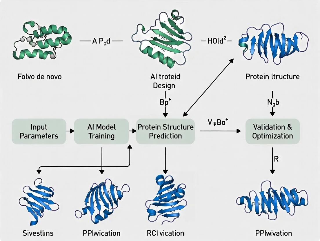
Visualizing the Workflow
(Diagram 1: AI-Driven De Novo Protein Design Workflow. Width: 760px)
The Scientist's Toolkit: Research Reagent Solutions
Table 2: Essential Reagents for De Novo Protein Workflows
| Item | Supplier Examples | Function in Protocol |
|---|---|---|
| Codon-Optimized Gene Fragments | Twist Bioscience, IDT | Provides high-fidelity DNA for de novo sequences not found in nature. |
| pET-28a(+) Expression Vector | Novagen/Merck | Standard, high-copy plasmid for T7-driven expression in E. coli. |
| Ni-NTA Superflow Cartridge | Qiagen | High-capacity immobilized metal affinity chromatography for His-tagged protein purification. |
| Superdex 75 Increase 10/300 GL | Cytiva | Size exclusion column for assessing monodispersity and final polishing. |
| Precision Protease (3C) | Thermo Fisher | Site-specific cleavage of fusion tags to yield native protein sequence. |
| Circular Dichroism Spectrophotometer | Applied Photophysics, Jasco | Measures secondary structure and thermal stability of purified proteins. |
This document details the integration of machine learning (ML) into the de novo protein design pipeline. The workflow shifts from a structure-centric approach to a sequence-first paradigm, where generative models propose novel protein sequences optimized for specific functions, which are then validated through high-throughput experimental loops.
Application Note 1: Generative Models for Protein Sequence Space Exploration
- Objective: To generate novel, foldable protein sequences targeting a specific functional site (e.g., an enzyme active site or a protein-protein interaction interface).
- Principle: Models like ProteinMPNN, RFdiffusion, and ESM-2 are trained on natural protein sequences and structures. They learn the complex mapping between local structural environments and amino acid preferences, enabling the in silico design of sequences that fold into desired backbone scaffolds.
- Key Advantage: Exponentially increases the diversity and quality of candidate sequences compared to traditional library-based methods (e.g., site-saturation mutagenesis).
Application Note 2: AlphaFold2 for In Silico Validation
- Objective: Rapid computational screening of ML-generated protein sequences for predicted structural integrity and folding fidelity.
- Principle: The designed sequences are fed into structure prediction engines (AlphaFold2, ESMFold). A high predicted confidence (pLDDT > 85-90) and congruence with the target backbone scaffold indicate a high probability of successful experimental expression and folding.
- Key Advantage: Filters out non-folders prior to costly synthesis and expression, dramatically improving experimental success rates.
Table 1: Quantitative Performance Metrics of Key ML Models in Protein Design
| Model | Primary Function | Key Metric | Reported Performance | Typical Runtime |
|---|---|---|---|---|
| ProteinMPNN | Sequence design for fixed backbones | Recovery of native-like sequences | ~52% sequence recovery on native backbones | Seconds per protein |
| RFdiffusion | De novo backbone generation | Designability (pLDDT) of outputs | >85% of designs with pLDDT > 80 | Minutes to hours |
| AlphaFold2 | Structure prediction | pLDDT (per-residue confidence) | >90 pLDDT for well-folded designs | Minutes per protein |
| ESMFold | High-speed structure prediction | TM-score to ground truth | Comparable to AF2, ~6x faster | Seconds to minutes |
Experimental Protocols
Protocol 1: De Novo Enzyme Design Using RFdiffusion and ProteinMPNN
Objective: Generate and validate a novel hydrolase enzyme for a target substrate.
Materials: See "Scientist's Toolkit" below.
Methodology:
- Motif Scaffolding: Define the functional motif (catalytic triad residues: Ser, His, Asp) in 3D space using RFdiffusion. Specify spatial constraints and generate 1,000 backbone scaffolds that spatially arrange these residues correctly.
- Sequence Design: For each generated backbone, use ProteinMPNN to design 5 sequences. Use conditional probabilities to fix the catalytic residues. This yields ~5,000 candidate sequences.
- In Silico Screening: Predict the structure of all 5,000 candidates using ESMFold/AlphaFold2. Filter based on:
- pLDDT > 85.
- Root-mean-square deviation (RMSD) of catalytic residue atoms < 1.0 Å from the target motif.
- Favorable binding pocket geometry around the substrate (assessed with molecular docking software like AutoDock Vina).
- Gene Synthesis & Cloning: Select the top 200 sequences for experimental testing. Order genes as pooled oligonucleotide libraries. Clone into an expression vector (e.g., pET-28b(+) using Gibson Assembly).
- High-Throughput Expression & Purification: Express in 96-well deep-well plates. Lyse cells and purify via His-tag using Ni-NTA plates.
- Activity Screening: Assay hydrolase activity using a fluorogenic substrate (e.g., 4-methylumbelliferyl ester) in a plate reader. Select hits with activity >3 standard deviations above negative control (scrambled sequence).
- Validation: Express and purify hits from step 6 at larger scale (50 mL). Determine kinetic parameters (kcat, KM) and validate structure via Size-Exclusion Chromatography (SEC) and/or X-ray crystallography.
Protocol 2: Iterative Affinity Maturation with Directed Evolution and ML
Objective: Improve the binding affinity of a designed protein binder.
Methodology:
- Initial Library Creation: Start with a parent ML-designed sequence. Generate a diverse variant library (~10^6 members) using error-prone PCR (epPCR) or a focused saturation mutagenesis library targeting predicted binding interface residues.
- Selection: Perform 2-3 rounds of yeast display or phage display against the biotinylated target antigen. Sort for binders using Fluorescence-Activated Cell Sorting (FACS).
- Sequence-activity Landscaping: Sequence all enriched variants (NGS, >10^4 reads). Train a simple supervised ML model (e.g., Gaussian Process Regression, shallow neural network) on the sequence-fitness data.
- Model-Guided Design: Use the trained model to virtually screen a massive mutational space (>10^8 variants). Select the top 50 predicted high-fitness sequences for synthesis and testing.
- Validation: Test purified variants for affinity using Biolayer Interferometry (BLI) or Surface Plasmon Resonance (SPR). Iterate back to step 1 if needed.
Visualization of Workflows & Pathways
Title: AI-Driven De Novo Protein Design Workflow
Title: ML-Guided Affinity Maturation Cycle
The Scientist's Toolkit: Research Reagent Solutions
| Item / Reagent | Function & Application in ML-Driven Protein Engineering |
|---|---|
| Oligo Pool Libraries (e.g., Twist Bioscience) | Provides cost-effective, high-fidelity synthesis of thousands of designed DNA sequences in parallel for high-throughput expression screening. |
| Gibson Assembly Master Mix | Enables seamless, one-pot cloning of pooled gene libraries into expression vectors without reliance on restriction sites. |
| Ni-NTA Magnetic Beads (96-well format) | Allows rapid, automated purification of His-tagged protein variants in high-throughput screening workflows. |
| Fluorogenic/Chromogenic Substrates | Enables sensitive, quantitative activity assays for enzymes in plate-based formats to score ML-designed variants. |
| Streptavidin Biosensors (for BLI) | Used for label-free, real-time kinetic analysis (kon, koff, KD) of protein binders during affinity maturation campaigns. |
| Yeast Display Vector (e.g., pYD1) | Platform for coupling genotype to phenotype in directed evolution, enabling FACS-based selection of binders for ML training. |
| Next-Generation Sequencing (NGS) Service | Provides deep sequencing of selection outputs, generating the sequence-fitness datasets required to train predictive ML models. |
| Structural Validation Kit (SEC column, Crystallization screen) | For final validation of designed proteins (monodispersity, 3D structure). |
Within the context of AI-driven de novo protein design, computational concepts bridge biophysical principles and machine learning. The workflow progresses from the physics-based calculation of molecular stability to the data-driven navigation of protein sequence and structure spaces. The fundamental pipeline moves from defining an Energy Function to scoring decoys, to sampling the Conformational Space, and finally to learning a compressed Latent Space for generative design.
Title: AI Protein Design Computational Pipeline
Key Concepts: Definitions, Data, and Quantitative Benchmarks
Table 1: Core Computational Concepts in Protein Design
| Concept | Mathematical Basis | Key Metrics (Typical Values) | Role in Protein Design |
|---|---|---|---|
| Energy Function (Force Field) | E_total = Σ bonds + Σ angles + Σ torsions + Σ vdW + Σ electrostatics + Σ solvation | Rosetta REF2015: AUC~0.7-0.8 for ΔΔG prediction; AlphaFold2 pLDDT >90 = high confidence | Provides a scoring landscape to discriminate stable vs. unstable structures. |
| Conformational Space | High-dimensional space of all possible backbone & side-chain coordinates. | For a 100-aa protein: ~10^100 possible conformations. Sampling efficiency: 10^3-10^6 decoys/design. | Defines the search problem; efficient sampling (MCMC, RL) is required to find low-energy states. |
| Latent Space (VAE/Diffusion) | z ~ Encoder(x), x' ~ Decoder(z); z ∈ ℝ^n (n=32-512). | Reconstruction loss (MSE) < 0.1; Perplexity of sequence generation; Diversity of generated structures. | Continuous, smooth representation enabling interpolation and optimization of protein properties. |
| Protein Language Model (pLM) Embedding | Contextual embedding from transformer models (e.g., ESM-2, ProtBERT). | ESM-2 embeddings (dim=1280) achieve >40% recovery rate in variant effect prediction. | Provides evolutionary-informed priors for sequence fitness, useful for scoring and conditioning. |
Table 2: Performance Comparison of Select Energy Functions & Generative Models (2022-2024)
| Method Name | Type | Key Benchmark Performance | Computational Cost (GPU hrs/design) |
|---|---|---|---|
| Rosetta REF2015 | Physics-based Energy Function | Successful de novo design of folds (TIM barrels, etc.), ΔΔG prediction RMSE ~1-2 kcal/mol. | High (100-1000s, CPU) |
| AlphaFold2 | Structure Prediction (Implicit Energy) | pLDDT >90 for high-confidence designs. Used for "inverse folding" validation. | Moderate (1-10, GPU) |
| RFdiffusion | Diffusion in Latent (Structural) Space | >50% experimental success rate on novel protein scaffolds (2023). | Low-Moderate (5-20, GPU) |
| ProteinMPNN | Inverse Folding (Sequence Design) | >2x recovery rate vs. Rosetta (∼50% vs. ∼20%) on native backbones. | Very Low (<0.1, GPU) |
| Chroma | Diffusion on Joint (Shape+Function) Space | Can condition on symmetry, function, yielding designed proteins with novel topology. | Moderate (10-50, GPU) |
Experimental Protocols
Protocol 1: Validating a Designed Protein Using a Composite Computational Pipeline Objective: To assess the stability and foldability of a de novo generated protein sequence before experimental characterization.
- Input: Generate initial candidate sequences using a generative model (e.g., RFdiffusion for backbone, ProteinMPNN for sequence).
- Energy Minimization: Relax the designed structure in a physics-based force field using the Rosetta
FastRelaxprotocol (200 cycles). - In-silico Folding: Use AlphaFold2 or ESMFold to predict the structure from the sequence ab initio.
- Command:
python run_alphafold.py --fasta_path design.fasta --output_dir ./af2_prediction
- Command:
- Structural Convergence Analysis: Calculate the Root Mean Square Deviation (RMSD) between the designed model and the in-silico folded prediction. Designs with RMSD < 2.0 Å are considered stable.
- Aggregation Propensity: Analyze using tools like
PISAorAggrescan3Dto check for exposed hydrophobic patches. - Output: A ranked list of designs with composite scores (Energy, pLDDT, RMSD, agg. score).
Protocol 2: Navigating a Latent Space for Property Optimization Objective: To generate novel protein sequences with high affinity for a target ligand by interpolating in a conditioned latent space.
- Model Setup: Use a conditional Variational Autoencoder (cVAE) or a diffusion model trained on protein structures/scaffolds with functional annotations.
- Define Conditioning Vector: Encode the desired property (e.g., a binding pocket shape from a target, a functional motif) into a conditioning vector
c. - Latent Space Interpolation:
- Sample two latent points
z1andz2from known functional proteins. - Linearly interpolate:
z' = α * z1 + (1-α) * z2, forαfrom 0 to 1. - Decode each
z'with the shared conditioncto generate novel backbone structures.
- Sample two latent points
- Sequence Design & Filtering: Use a fast inverse folding model (ProteinMPNN) to design sequences for each interpolated backbone.
- Property Prediction: Score designs using a docking simulation (e.g., with Rosetta
FlexDockorAutoDock Vina) to estimate binding affinity. - Iterate: Use the scores as feedback to refine the search in latent space (e.g., via Bayesian optimization).
The Scientist's Toolkit: Research Reagent Solutions
Table 3: Essential Computational Tools for AI-Driven Protein Design (2024)
| Item/Tool Name | Category | Function in Workflow |
|---|---|---|
| PyRosetta | Energy Function & Sampling | Python interface to the Rosetta software suite. Used for detailed energy minimization, docking, and design calculations. |
| AlphaFold2 (ColabFold) | Structure Prediction | Provides rapid, accurate structure prediction from sequence to validate de novo designs (via pLDDT confidence score). |
| RFdiffusion | Generative Model (Structure) | Generates novel protein backbones conditioned on symmetry, shape, or functional site constraints. |
| ProteinMPNN | Inverse Folding | Robustly designs sequences for fixed backbones, significantly higher success rates than previous methods. |
| ESM-2/ESMFold | Protein Language Model | Provides evolutionary-scale sequence embeddings and fast, reasonable-accuracy structure prediction for high-throughput screening. |
| ChimeraX / PyMOL | Visualization & Analysis | Critical for 3D visualization of designed models, analyzing interfaces, and preparing figures. |
| MD Simulation (GROMACS/OpenMM) | Molecular Dynamics | Used for in-silico stability assessment via nanosecond-scale simulations to check for unfolding. |
| JAX / PyTorch (with GPU) | Deep Learning Framework | Essential for developing, fine-tuning, or running custom generative models and neural networks in the design pipeline. |
Workflow Visualization: AI-DrivenDe NovoDesign
Title: AI Protein Design and Evaluation Workflow
Application Notes: AI-Driven De Novo Design Pipeline
The integration of artificial intelligence, particularly deep learning-based structure prediction (AlphaFold2, RosettaFold) and generative models (ProteinMPNN, RFdiffusion), has revolutionized de novo protein design. This workflow enables the rapid creation of proteins with tailored functions for therapeutic, catalytic, and material applications, moving beyond natural protein scaffolds.
Therapeutics: De Novo Mini-Binders
AI-designed proteins can target previously "undruggable" epitopes on pathogenic proteins or cell surface receptors. Mini-binders offer advantages over traditional antibodies, including greater stability, smaller size for tissue penetration, and ease of production.
- Key Case Study (2023): Design of high-affinity mini-binders against conserved epitopes of influenza hemagglutinin and SARS-CoV-2 spike protein variants. These binders neutralized the virus by blocking host cell receptor engagement.
- Quantitative Data Summary:
| Application | Designed Protein | Target | Affinity (K_D) | Key Metric (e.g., IC50, Stability) | Reference Year |
|---|---|---|---|---|---|
| Antiviral | HB36.6 (de novo) | Influenza H1 Hemagglutinin | 30 nM | Neutralization IC50: 12 nM | 2023 |
| Oncology | ProBind-IL2Rα | CD25 (IL-2 Receptor α) | 1.2 nM | Inhibits Treg cell signaling in vitro | 2024 |
| Anti-toxin | DeNovo-ToxinA | C. difficile Toxin B | 45 pM | Protects in murine challenge model | 2023 |
Enzymes: Designed Catalysts
Generative models are used to scaffold functional active sites, creating enzymes for non-natural reactions or improving the kinetics and stability of existing biocatalysts for industrial synthesis.
- Key Case Study (2024): Design of a "Kemp eliminase" with a catalytic efficiency (kcat/KM) exceeding 10^6 M⁻¹s⁻¹, rivaling natural enzymes, for a key organic synthesis step.
- Quantitative Data Summary:
| Enzyme Class | Designed For Reaction | Catalytic Efficiency (kcat/KM) | Thermostability (Tm) | Turnover Number (k_cat) | Reference Year |
|---|---|---|---|---|---|
| Hydrolase | PET plastic degradation | 580 s⁻¹M⁻¹ | 72 °C | 25 s⁻¹ | 2023 |
| Lyase | Kemp Elimination | 1.4 x 10^6 M⁻¹s⁻¹ | 68 °C | 450 s⁻¹ | 2024 |
| Transferase | Non-natural C-N bond formation | 320 s⁻¹M⁻¹ | 61 °C | 5.2 s⁻¹ | 2023 |
Novel Biomaterials: Self-Assembling Nanostructures
AI models guide the design of protein monomers that predictably self-assemble into filaments, cages, or 2D layers with atomic-level precision, enabling new drug delivery vehicles and catalytic scaffolds.
- Key Case Study (2023): Design of a tetrahedral protein nanocage with precisely controllable porosity (8 nm internal cavity) for encapsulating CRISPR-Cas9 ribonucleoproteins.
- Quantitative Data Summary:
| Material Type | Primary Function | Key Dimension/Property | Assembly Yield | Application Demonstrated | Reference Year |
|---|---|---|---|---|---|
| Nanocage (T=3) | Molecular Encapsulation | 25 nm outer diameter, 8 nm cavity | >85% | Cas9 RNP delivery | 2023 |
| 2D Protein Layer | Sensing/ Catalysis | Pore size: 2.3 nm, lattice const: 9.1 nm | N/A | Conductivity sensor | 2024 |
| Protein Filament | Scaffolding | Diameter: 10 nm, tunable length | >90% | Tissue engineering scaffold | 2023 |
Detailed Experimental Protocols
Protocol 1:De NovoMini-Binder Design & Validation
AIM: Generate and characterize a high-affinity binder against a flat protein-protein interaction interface.
Materials: See "The Scientist's Toolkit" below.
METHOD:
- Target Selection & Epitope Specification: Define target protein (e.g., viral spike). Use structural data (PDB, AF2 prediction) to select a conserved, solvent-accessible epitope.
- Scaffold Generation with RFdiffusion:
- Input: Epitope residues as "motif" constraints.
- Parameters:
contigmap.contigs=[A/80-100](design chain length),ppi.hotspot_res=[list of epitope residue indices]. - Run diffusion sampling to generate 1,000-10,000 backbone scaffolds placing binder N/C termini near epitope edges.
- Sequence Design with ProteinMPNN:
- Input: Selected backbone scaffolds (top 100 by pLDDT).
- Parameters:
fixed_pos=[list of epitope residue indices],chain_letters='A'. - Output: Generate 128 sequences per scaffold. Filter for natural amino acid probability >0.7.
- In Silico Affinity Screening:
- Fold all designed sequences (AlphaFold2 multimer) in complex with the target.
- Calculate interface pTM (ipTM) and interface PAE (predicted Aligned Error). Select top 50 designs with ipTM >0.7 and low interface PAE.
- Perform molecular dynamics (MD) simulation (50 ns) to assess complex stability. Rank by RMSD and binding free energy (MM/PBSA).
- In Vitro Expression & Purification (Top 10 Designs):
- Clone genes into pET-28a(+) vector, transform BL21(DE3) E. coli.
- Express in 1L Terrific Broth with 0.5 mM IPTG at 18°C for 18h.
- Purify via Ni-NTA affinity chromatography, followed by size-exclusion chromatography (Superdex 75 Increase 10/300 GL) in PBS, pH 7.4.
- Biophysical Characterization:
- SEC-MALS: Confirm monomeric state.
- BLI/Bio-Layer Interferometry: Load biotinylated target onto Streptavidin biosensors. Measure binding kinetics of serially diluted binders (100 nM to 1.56 nM). Fit data to 1:1 binding model to obtain KD, kon, koff.
- DSC (Differential Scanning Calorimetry): Determine melting temperature (Tm) at 1°C/min scan rate.
Protocol 2: Characterization of aDe NovoEnzyme
AIM: Express and kinetically characterize an AI-designed enzyme.
METHOD:
- Expression & Purification: Follow steps in Protocol 1.5. Use appropriate buffer for enzyme activity (e.g., 50 mM Tris, 150 mM NaCl, pH 8.0).
- Initial Activity Screen: Perform endpoint assay with high substrate concentration (10 x predicted K_M) and 1 µM enzyme at 25°C for 10 min. Detect product formation (absorbance/fluorescence) compared to negative control (no enzyme).
- Steady-State Kinetics:
- Prepare substrate in 8 concentrations (0.2x to 5x predicted KM).
- Dilute enzyme to working concentration (typically 10-100 nM).
- In a 96-well plate, mix 50 µL substrate with 50 µL enzyme to start reaction. Monitor initial velocity (V0) for 2-5 min.
- Fit [S] vs. V0 data to the Michaelis-Menten equation using non-linear regression (GraphPad Prism) to extract kcat and K_M.
- Thermal Stability Assay (TSA):
- Use a real-time PCR instrument. Mix 25 µL of 2 µM enzyme with 25 µL of 10X SYPRO Orange dye in buffer.
- Run a temperature ramp from 25°C to 95°C at 1°C/min, monitoring fluorescence.
- Determine T_m as the inflection point of the fluorescence vs. temperature curve.
Diagrams & Workflows
AI Protein Design & Test Cycle
Enzyme Catalytic Cycle (Michaelis-Menten)
The Scientist's Toolkit: Research Reagent Solutions
| Item / Reagent | Supplier Examples | Function in AI Protein Workflow |
|---|---|---|
| RFdiffusion & ProteinMPNN (Software) | Robetta Server, GitHub Repos | Core generative AI models for backbone design and sequence optimization. |
| AlphaFold2 Multimer (Colab/Server) | ColabFold, Local Installation | Predicts 3D structure of designed protein monomers and complexes with targets. |
| pET-28a(+) Vector | Novagen, MilliporeSigma | Standard T7 expression vector with N-terminal His-tag for bacterial protein production. |
| BL21(DE3) Competent Cells | NEB, Thermo Fisher | E. coli strain for high-yield, IPTG-induced expression of recombinant proteins. |
| Ni-NTA Superflow Resin | Qiagen, Cytiva | Immobilized metal affinity chromatography resin for purifying His-tagged proteins. |
| Superdex 75 Increase (SEC Column) | Cytiva | Size-exclusion chromatography column for polishing and buffer exchange of proteins <70 kDa. |
| Octet RED96e System (BLI) | Sartorius | Label-free biosensor platform for real-time measurement of binding kinetics (KD, kon, k_off). |
| SYPRO Orange Dye | Thermo Fisher | Fluorescent dye used in thermal shift assays (TSA) to determine protein melting temperature (T_m). |
| Precision Plus Protein Standards | Bio-Rad | Molecular weight markers for SDS-PAGE analysis of protein purity and size. |
Application Notes
For a robust AI-driven de novo protein design workflow, three foundational pillars must be established before initiating design cycles. These prerequisites are interdependent; weaknesses in one compromise the efficacy of the entire pipeline.
1. Data: The Empirical Substrate The quality, quantity, and relevance of biological data directly determine the learnable universe of an AI model. For de novo design, this extends beyond structural databases to include evolutionary, biophysical, and functional information.
2. Domain Knowledge: The Interpretive Framework Computational predictions require experimental grounding. Domain knowledge in structural biology, biophysics, and biochemistry is critical for formulating design problems, curating training data, interpreting model outputs, and prioritizing designs for experimental validation.
3. Computational Resources: The Execution Engine The scale of modern protein design models demands significant hardware and software infrastructure. Resource allocation must align with the chosen model's architecture and the intended throughput of the design-test-learn cycle.
Table 1: Core Data Resources for AI-Driven Protein Design
| Data Type | Primary Source(s) (as of 2024) | Key Metrics (Approx. Volume) | Primary Use in Workflow |
|---|---|---|---|
| Protein Structures | Protein Data Bank (PDB), AlphaFold DB | ~250,000 (PDB); ~200 million (AF DB) | Training structure-predicting/designing models; template identification. |
| Protein Sequences | UniProt, NCBI GenPept | ~250 million sequences (UniProt) | Learning evolutionary constraints, sequence-structure relationships. |
| Structural Motifs & Folds | CATH, SCOP, ECOD | ~5,000 folds, ~130,000 superfamilies | Providing architectural templates and classifying design outputs. |
| Protein-Protein Interactions | BioGRID, STRING, PDB complexes | Millions of interactions | Designing binders, interfaces, and multi-component assemblies. |
| Biophysical & Stability Data | ThermoMutDB, ProTherm, literature | ~100,000+ mutant stability entries | Fine-tuning models for stability, refining energy functions. |
Experimental Protocols
Protocol 1: Curating a High-Quality Training Dataset for a Conditional Protein Design Model Objective: To assemble a non-redundant, labeled dataset of protein structures and sequences for training a neural network to generate sequences conditioned on a desired fold or function.
Source Data Retrieval:
- Download the latest PDB release. Filter entries for experimental resolution ≤ 3.0 Å and remove nucleic acid-only structures.
- Extract corresponding sequences from the PDB headers or cross-reference with UniProt IDs.
Redundancy Reduction & Clustering:
- Use MMseqs2 (sequence-based) or CD-HIT (sequence-based) to cluster protein chains at 30% sequence identity.
- Select a representative chain from each cluster (e.g., the highest resolution structure).
Annotation & Labeling:
- For each representative structure, generate labels using external databases:
- Fold Label: Run Foldseck against the PDB to assign a CATH or ECOD classification.
- Functional Label: Map to Gene Ontology (GO) terms via the SIFTS service or UniProt cross-references.
- Parse structures into backbone coordinates (N, Cα, C, O atoms) and convert residues to one-hot encoded sequence vectors.
- For each representative structure, generate labels using external databases:
Dataset Splitting:
- Perform splits at the cluster level (not individual chain) to prevent data leakage. Use an 80/10/10 ratio for training, validation, and test sets.
Protocol 2: In Silico Validation Pipeline for Generated Protein Designs Objective: To computationally triage and rank de novo generated protein designs prior to wet-lab experimentation.
Structure Prediction & Self-Consistency:
- Input the AI-generated sequence into AlphaFold2 or RoseTTAFold (local installation or via API).
- Align the predicted structure (AF/RTF output) with the design target (e.g., the intended backbone from the model). Calculate the Root-Mean-Square Deviation (RMSD) of Cα atoms.
- Designs with low RMSD (< 2.0 Å) pass this initial fold-recovery check.
Energy-Based Scoring:
- Subject the predicted structure to all-atom refinement using Rosetta relax.
- Calculate Rosetta's total_score and ddG (estimated stability) for the design. Filter out designs with poor scores indicative of folding instability.
Aggregate Scoring & Ranking:
- Create a composite score: Z = (w1 * RMSD) + (w2 * total_score) + (w3 * ddG). Weights (w1, w2, w3) are negative for metrics where lower is better.
- Rank all designs by composite score Z. Top-ranking designs proceed to in vitro testing.
Visualizations
Diagram 1: Prerequisite Interdependence in AI Protein Design
Diagram 2: Pre-Experimental Design Validation Workflow
The Scientist's Toolkit
Table 2: Essential Research Reagent Solutions & Computational Tools
| Tool/Reagent | Category | Primary Function in Workflow |
|---|---|---|
| AlphaFold2/ColabFold | Software | Provides rapid, accurate structure prediction for both natural and designed sequences, enabling fold-recovery validation. |
| PyRosetta | Software | A Python-accessible library for the Rosetta suite. Used for energy scoring, structural refinement, and computational mutagenesis. |
| MMseqs2 | Software | Enables fast, sensitive clustering of massive sequence datasets for redundancy reduction and homology detection. |
| CATH/ECOD Database | Database | Provides hierarchical, manually curated classification of protein domains, essential for labeling training data and analyzing design novelty. |
| Gene Fragments (gBlocks, etc.) | Wet-Lab Reagent | Synthetic double-stranded DNA fragments for cost-effective codon-optimized synthesis of de novo protein sequences for expression testing. |
| High-Throughput Cloning Kit (e.g., Gibson Assembly) | Wet-Lab Reagent | Enables parallel assembly of dozens to hundreds of designed gene constructs into expression vectors. |
| Differential Scanning Fluorimetry (DSF) Dyes | Wet-Lab Reagent | Fluorescent dyes (e.g., SYPRO Orange) used in thermal shift assays to rapidly estimate protein stability and folding of purified designs. |
| NVIDIA A100/H100 GPU | Hardware | Specialized processing units essential for training large protein language or diffusion models and for high-throughput inference. |
Building from Scratch: A Step-by-Step AI-Driven Protein Design Pipeline
Within AI-driven de novo protein design research, Phase 1 is the critical translational bridge between a conceptual biological problem and a computationally tractable design goal. This phase defines the target protein's functional, structural, and biophysical parameters, constraining the vast sequence space for subsequent generative AI models. A precise specification prevents resource-intensive cycles of generation and experimental validation of non-functional designs.
Core Components of Problem Definition
A comprehensive problem definition addresses four pillars:
Table 1: Core Components of Problem Definition
| Component | Description | Example Specification for a Therapeutic Enzyme |
|---|---|---|
| Primary Function | The central biochemical activity the protein must perform. | Catalyze hydrolysis of peptide bond between residues X and Y in Target Protein Z. |
| Target & Context | The molecular target, cellular environment, or application. | Function in human plasma (pH 7.4, 150 mM NaCl, 37°C) against soluble Target Z. |
| Success Metrics & Assays | Quantitative benchmarks for in vitro and in silico validation. | kcat/KM > 1 x 10⁴ M⁻¹s⁻¹; Thermal stability (Tm) > 60°C; Expression yield > 5 mg/L in E. coli. |
| Constraint & Negatives | Undesired characteristics or off-target activities to be avoided. | No proteolytic activity against human serum albumin; Size < 50 kDa. |
From Problem to Functional Specification
The functional specification translates the definition into explicit, engineerable parameters for AI model conditioning.
Table 2: Elements of the Functional Specification
| Specification Domain | Key Parameters | AI/Design Implication |
|---|---|---|
| Structural | Fold (e.g., TIM barrel, Ig-like), symmetry (monomer/oligomer), approximate dimensions. | Conditions geometric deep learning models; defines folding landscape. |
| Functional Site | Catalytic residue identities (e.g., Ser-His-Asp triad), metal coordination, binding pocket volume/shape, co-factor requirement. | Directs focused sequence generation around active site; defines binding energy objectives. |
| Biophysical | Target stability (ΔG of folding), pI, hydrophobicity profile, aggregation propensity (e.g., low Zyggregator score). | Sets Rosetta/D-AlphaFold energy function weights or discriminator thresholds in generative AI. |
| Expressibility | Host organism (e.g., E. coli, CHO cells), codon optimization flag, purification tag requirement (e.g., His6). | Informs final sequence post-processing and experimental planning. |
Experimental Protocols for Specification Validation
Prior to full-scale design, preliminary experiments validate assumptions about the target and function.
Protocol 4.1: Target Interaction Profiling via Surface Plasmon Resonance (SPR) Purpose: To characterize the kinetics and affinity of a natural ligand/target interaction, setting benchmarks for designed binders. Materials: See Scientist's Toolkit. Method:
- Surface Preparation: Immobilize the target protein on a CMS sensor chip via amine coupling to achieve ~100 Response Units (RU).
- Binding Kinetics: Run a concentration series (e.g., 0.1 nM to 1 µM) of the natural ligand in HBS-EP buffer (10 mM HEPES, 150 mM NaCl, 3 mM EDTA, 0.005% v/v Surfactant P20, pH 7.4) at a flow rate of 30 µL/min.
- Regeneration: Dissociate bound ligand with a 30-second pulse of 10 mM glycine-HCl (pH 2.0).
- Data Analysis: Fit the resulting sensorgrams to a 1:1 Langmuir binding model using the Biacore Evaluation Software to extract association (kon) and dissociation (koff) rates. Calculate equilibrium dissociation constant KD = koff/kon.
Protocol 4.2: Orthogonal Assay Development for Functional Screening Purpose: Establish a robust, medium-throughput assay to test designed protein function. Example – Enzymatic Activity:
- Substrate Preparation: Source or synthesize a fluorogenic or chromogenic substrate mimicking the natural target (e.g., a peptide with a quenched fluorophore).
- Assay Optimization: In a 96-well plate, titrate substrate concentration (1 µM to 1 mM) against a fixed concentration of positive control enzyme in reaction buffer.
- Signal Detection: Measure fluorescence/absorbance change kinetically over 30 minutes using a plate reader.
- Validation: Calculate Z'-factor using positive (enzyme + substrate) and negative (substrate only) controls. A Z' > 0.5 indicates a robust assay for screening.
Mandatory Visualizations
Diagram 1: Phase 1 Workflow Logic
Diagram 2: Functional Specification Inputs for AI
The Scientist's Toolkit: Research Reagent Solutions
Table 3: Key Reagents for Specification & Validation
| Reagent/Material | Vendor Examples (2024) | Function in Phase 1 |
|---|---|---|
| Biacore Series S Sensor Chip CMS | Cytiva | Gold-standard SPR surface for kinetic analysis of protein-protein interactions. |
| Fluorogenic Peptide Substrates | Bachem, GenScript, custom synthesis | Enable sensitive, continuous activity assays for enzymes (proteases, kinases). |
| Stability Dyes (e.g., SYPRO Orange) | Thermo Fisher Scientific | Used in differential scanning fluorimetry (nanoDSF) to measure protein thermal melting (Tm). |
| HEK293F or CHO Transient Expression System | Thermo Fisher, Sartorius | Mammalian expression platform for testing expression of designs requiring disulfides or glycosylation. |
| Codon-Optimized Gene Fragments (clonal DNA) | Twist Bioscience, Integrated DNA Technologies | Rapid, high-fidelity source of DNA for constructing expression vectors for test designs. |
| Affinity Purification Resins (Ni-NTA, Streptactin) | Qiagen, IBA Lifesciences | For reliable, standardized purification of His-tagged or Strep-tagged test proteins. |
Application Notes
In the context of AI-driven de novo protein design workflow research, the selection and orchestration of generative models constitute the critical second phase. This phase transforms initial structural hypotheses into viable, sequence-specific protein designs. The current paradigm leverages a synergistic pipeline where diffusion-based backbone generation is followed by sequence design and rigorous validation. This section details the application notes for three cornerstone tools: RFdiffusion for structure generation, ProteinMPNN for sequence design, and AlphaFold2 for in silico validation.
RFdiffusion, developed by the Baker Lab, is a generative model built upon a RoseTTAFold architecture that applies diffusion probabilistic models to protein backbone coordinates. It iteratively denoises a 3D structure from random noise, conditioned on user-defined constraints (e.g., symmetric assemblies, motif scaffolding, binder design). Its primary output is all-atom protein backbones (Cα, C, N, O atoms) with placeholder sidechains.
ProteinMPNN, also from the Baker Lab, is a message-passing neural network for solving the inverse folding problem. Given a backbone structure (e.g., from RFdiffusion), it predicts optimal amino acid sequences that stabilize that fold. It offers high-speed, high-accuracy sequence design with controllable features like fixed sequence regions or temperature-based diversity sampling.
AlphaFold2, from DeepMind, serves as the de facto standard for structure validation within the design pipeline. By predicting the structure of a ProteinMPNN-designed sequence, it provides a critical "folding confidence" check. A high agreement between the designed (input) backbone and the AlphaFold2-predicted structure (pLDDT > 85, TM-score > 0.8) indicates a design with high native-state plausibility.
Quantitative Performance Comparison: The table below summarizes key metrics for model selection.
Table 1: Comparative Performance Metrics for Generative Models
| Model (Primary Task) | Key Metric | Typical Performance Range | Runtime (CPU/GPU) | Key Conditioning Inputs |
|---|---|---|---|---|
| RFdiffusion (Backbone Gen.) | Design Success Rate* | 10-50% (highly task-dependent) | Hours (GPU) | Symmetry, Motifs, Binder Site |
| ProteinMPNN (Sequence Design) | Recovery Rate | ~40-60% on native backbones | Seconds/backbone (GPU) | Backbone coords., Fixed residues |
| AlphaFold2 (Validation) | pLDDT / TM-score | pLDDT > 85 (High conf.) | Minutes (GPU) | Amino Acid Sequence |
Success rate defined by experimental expression, stability, or functional activity in downstream assays. *Recovery of native sequence when given native backbone.
Experimental Protocols
Protocol 1:De NovoScaffold Generation with RFdiffusion
Objective: Generate a novel protein backbone structure scaffolding a specified functional motif.
- Input Preparation: Define the target functional motif as a PDB file containing Cα coordinates. Create a YAML configuration file specifying the task (e.g.,
partial_diffusionfor motif scaffolding), the path to the motif PDB, and which chains are fixed. - Model Configuration: Download the pre-trained RFdiffusion model weights (v1.1 or later). Set the inference parameters:
num_designs=100,steps=100(for motif scaffolding), andcontigsstring defining the variable scaffold region (e.g.,A/10-50/0). Execution: Run the inference script. Example command:
Output Processing: The output directory will contain PDB files for each designed backbone. Cluster the backbones using RMSD-based clustering (e.g., with MMseqs2) to select topologically distinct representatives (typically 5-10 clusters).
Protocol 2: Fixed-Backbone Sequence Design with ProteinMPNN
Objective: Design stable, foldable amino acid sequences for a given backbone structure.
- Backbone Input: Use the selected RFdiffusion-generated PDB file(s). Ensure the file contains only backbone atoms (N, Cα, C, O) or full atoms with sidechains to be redesigned.
- Parameter Setup: Choose the ProteinMPNN model variant (
v_48_020recommended). Setnum_seq_per_target=200,sampling_temp=0.1(low for conservative designs) or0.3(for diverse sequences). Specify any fixed positions (e.g., motif residues) via a chain-and-residue list. Execution: Run the ProteinMPNN design script.
Sequence Selection: The output JSON file contains sequences ranked by log likelihood. Select the top 20-50 sequences for validation. Optionally, filter sequences using metrics like net charge or hydrophobicity to meet biophysical criteria.
Protocol 3:In SilicoFolding Validation with AlphaFold2
Objective: Assess the foldability of ProteinMPNN-designed sequences and their structural fidelity to the design target.
- Environment Setup: Install AlphaFold2 (v2.3.1 or later) with required databases. For high-throughput, use the stripped-down
alphafold-fastversion or ColabFold. Batch Prediction: Prepare a FASTA file containing the selected ProteinMPNN-designed sequences. Run AlphaFold2 in inference mode with reduced recycles (
--num_recycle=3) for speed, as this is a screening step.Analysis: For each design, extract the predicted aligned error (PAE) and pLDDT from the output JSON. Calculate the TM-score between the designed backbone (Protocol 1) and the AlphaFold2-predicted structure using tools like US-align. Selection Criterion: Proceed designs with pLDDT > 85 and TM-score (design vs. AF2 prediction) > 0.8 to the next workflow phase (experimental characterization).
Workflow Diagram
Diagram Title: AI Protein Design Phase 2: Generative Model Pipeline
The Scientist's Toolkit
Table 2: Essential Research Reagents & Computational Tools
| Item | Function in Workflow | Example / Specification |
|---|---|---|
| RFdiffusion Model Weights | Pre-trained neural network parameters for conditional backbone generation. | Downloaded model file (e.g., RFdiffusion.pt). |
| ProteinMPNN Model Weights | Pre-trained neural network for inverse folding/sequence design. | Model variant v_48_020 or v_48_002. |
| AlphaFold2 Database | Structural and sequence databases for MSA and template search. | BFD, MGnify, PDB70, Uniref30 (approx. 2.2TB total). |
| High-Performance GPU | Accelerates neural network inference for all three models. | NVIDIA A100 or V100 (32GB+ VRAM recommended). |
| Cluster Software (MMseqs2) | For clustering designed backbones or sequences to select diverse candidates. | MMseqs2 easy-cluster module. |
| Structural Alignment Tool | Computes TM-score/RMSD between designed and predicted structures. | US-align or PyMOL alignment scripts. |
| PDB File Format | Standard format for input (motifs) and output (backbones) structures. | Protein Data Bank file format, backbone atoms only. |
| FASTA File Format | Standard format for input/output of amino acid sequences. | Text file with > header followed by sequence. |
Within the context of an AI-driven de novo protein design workflow, Phase 3 represents the core generative engine. This phase translates abstract functional specifications and structural blueprints from prior phases into explicit, plausible protein sequences and their corresponding three-dimensional structures. The efficacy of the entire pipeline hinges on the sophisticated sampling strategies employed here, which balance exploration of the vast sequence-structure space with the exploitation of known biophysical principles.
Foundational Models & Data
Key Generative Models
Modern sequence and structure generation leverages deep generative models trained on the evolutionary and structural record of the Protein Data Bank (PDB) and associated sequence databases.
Table 1: Primary Generative Models for De Novo Design
| Model Name | Core Architecture | Primary Output | Key Strength | Typical Application in Phase 3 |
|---|---|---|---|---|
| ProteinMPNN | Message Passing Neural Network | Optimal sequences for a given backbone | High speed, state-of-the-art recovery rates | Fixed-backbone sequence design |
| RFdiffusion | Diffusion Model (RoseTTAFold backbone) | Novel protein backbone structures | Controllable generation of symmetric, binder, or motif-scaffolded structures | Unconstrained de novo backbone generation |
| AlphaFold2 | Evoformer & Structure Module | Predicted structure for a given sequence | Unparalleled accuracy in structure prediction | In silico validation of designed sequences |
| ESM-2/ESMFold | Large Language Model (Transformer) | Sequence embeddings & structure prediction | Captures deep evolutionary constraints; fast inference | Sequence generation & initial structure validation |
| Chroma | Diffusion Model on SE(3) manifold | Joint sequence-structure generation | Unified generative process for sequence and structure | End-to-end unconditional/conditional generation |
Experimental Protocol: Fixed-Backbone Sequence Design with ProteinMPNN
Protocol 3.1: High-Throughput Sequence Design for a Scaffold Objective: Generate diverse, low-energy amino acid sequences compatible with a predetermined backbone structure (from Phase 2).
Materials:
- Input: PDB file of target backbone (scaffold).
- Software: Local or cloud-based ProteinMPNN installation (PyTorch).
- Hardware: GPU (e.g., NVIDIA A100, 16GB+ VRAM recommended).
Procedure:
- Preprocessing: Prepare the input PDB file. Define designable positions (e.g., all residues, or only those within a functional pocket). Optionally, specify residue constraints (e.g., fix catalytic triad residues).
- Model Configuration: Set ProteinMPNN parameters:
model_type: 'v48020' (trained with more data).num_seq_per_target: 500 (number of sequences to generate).sampling_temperature: 0.1 (lower for greedy, higher for diversity).seed: [Integer] for reproducibility.batch_size: Adjust based on GPU memory.
- Execution: Run the ProteinMPNN script. The model performs autoregressive decoding from C- to N-terminus, conditioning the probability of each residue on the backbone structure and previously decoded residues.
- Output: A FASTA file containing 500 designed sequences, with a per-residue log-likelihood score for each.
Expected Results: A set of sequences predicted to fold into the input backbone. Top designs typically have negative log-likelihoods (higher probability).
Experimental Protocol:De NovoBackbone Generation with RFdiffusion
Protocol 3.2: Controllable Backbone Generation via Diffusion Objective: Generate novel, stable protein backbone structures that incorporate a desired motif or comply with symmetry constraints.
Materials:
- Input: (Conditional) PDB of motif or symmetry specification (e.g., C3 symmetry axis).
- Software: RFdiffusion codebase, PyRosetta or AlphaFold2 for validation.
- Hardware: High-memory GPU (NVIDIA A100 40GB+ recommended).
Procedure:
- Conditioning Setup: Define the generation objective via flags:
- Unconditional:
inference.num_designs=100 - Symmetric oligomer:
contigmap.contigs=[A/100-150]+symmetry.G=symmetry_group(e.g., C3). - Motif scaffolding:
contigmap.contigs=[A/80-100/0 10-30/A/40-60]to scaffold a motif (residues 10-30 of chain A).
- Unconditional:
- Diffusion Process: Execute the inference script. The model starts from pure Gaussian noise and iteratively denoises over a set number of steps (e.g., 50), guided by the conditioning input and the trained neural network.
- Truncation & Output: The final denoised backbone coordinates are extracted. Multiple independent runs yield diverse scaffolds.
- Initial Filtering: Filter outputs based on predicted TM-score to the condition (if applicable) and intra-backbone clashes.
Expected Results: A set of novel backbone PDB files. For motif scaffolding, the specified motif will be embedded within a novel, surrounding structure.
Sampling Strategies & Search Algorithms
The generative model provides a distribution; sampling strategies determine how designs are drawn from it.
Table 2: Sampling Strategies for Sequence-Structure Generation
| Strategy | Description | Control Parameters | Advantage | Disadvantage |
|---|---|---|---|---|
| Greedy Decoding | Selects the highest probability residue at each step. | temperature=0.1 |
Produces the single most probable sequence. Ignores diversity. | No exploration; may get stuck in local minima. |
| Temperature Sampling | Samples from a softened probability distribution. | temperature (0.1-1.0) |
Tunes diversity vs. probability. Higher T increases exploration. | Can produce lower-fitness sequences. |
| Markov Chain Monte Carlo (MCMC) | Proposes sequence changes, accepts/rejects based on energy function. | Step count, cooling schedule | Can escape local optima; converges to target distribution. | Computationally expensive; requires careful tuning. |
| Inpainting/Masked Sampling | Masks a portion of the sequence/structure, infers it conditioned on context. | Mask ratio, number of iterations | Enables local exploration around a stable framework. | Limited global exploration. |
| Directed Evolution In Silico | Uses generative model to propose mutations, filtered by a fitness predictor. | Rounds of mutation, selection pressure | Directly optimizes for a downstream functional property. | Requires a reliable fitness oracle (e.g., a classifier). |
Visualization of Workflows
Diagram 1: AI-Driven Sequence & Structure Generation Pipeline
Diagram 2: Decision Logic for Sampling Strategy Selection
The Scientist's Toolkit
Table 3: Research Reagent Solutions for Phase 3 Validation
| Item | Function in Phase 3 | Example/Supplier Notes |
|---|---|---|
| PyRosetta | Computational suite for energy scoring, structural perturbation (minimization, docking), and detailed biophysical analysis. Used to relax designed structures and calculate metrics like ddG (ΔΔG). | License required. RosettaScripts enable custom protocols. |
| AlphaFold2 (ColabFold) | Provides a rapid, accurate in silico validation step. The predicted structure for a designed sequence should closely match the intended generative model output. | Local installation or via ColabFold for batch processing. |
| Phenix (pdb_tools, MolProbity) | Suite for structural analysis. Used to validate geometry (Ramachandran plots, rotamer outliers, clashscore) of generated models. | Open source. Critical for pre-experimental filtering. |
| ESM-2 (650M params) | Provides sequence embeddings used as features for downstream classifiers (e.g., for predicting stability or function). Also used for fast, albeit less accurate, structure prediction via ESMFold. | Hugging Face Transformers library. |
| MD Simulation Software (GROMACS, OpenMM) | Performs short, restrained molecular dynamics simulations to assess local stability and side-chain packing of designed proteins. | Requires HPC resources. Used for deeper validation of top candidates. |
| Custom Python Scripts (BioPython, PyMOL Scripting) | Essential for pipeline automation: parsing PDB/FASTA files, batch running tools, extracting metrics, and generating reports. | Open-source libraries form the glue of the workflow. |
In this phase of the AI-driven de novo protein design workflow, computationally generated protein candidates are rigorously filtered and evaluated for structural stability and developability. This stage is critical for translating vast numbers of AI-generated sequences into a shortlist of viable constructs for experimental characterization, significantly reducing time and resource expenditure.
Core Filtering Criteria and Protocols
Sequence-Based Filtering
Objective: Remove sequences with undesirable biochemical properties. Protocol:
- Input the FASTA file of AI-generated candidate sequences.
- Calculate the following metrics for each sequence using Biopython or custom scripts:
- Length: Discard sequences deviating >±10% from the target length.
- Amino Acid Composition: Flag sequences with unusual residue frequencies (e.g., >25% hydrophobic residues for soluble targets).
- Charge and pI: Calculate isoelectric point (pI) using the Bjellqvist method. Filter based on target solubility requirements (e.g., pI 5-9 for reduced aggregation).
- Instability Index: Compute using the method of Guruprasad et al. (1990). Sequences with an index >40 are considered unstable.
- Sequence Complexity: Remove low-complexity sequences using the SEG algorithm.
- Output a filtered FASTA file.
Structural Stability Prediction via Deep Learning
Objective: Predict the folded state stability of candidate structures. Protocol (Using AlphaFold2 or RoseTTAFold for Structural Generation):
- Submit the filtered sequences from 2.1 to a local or cloud-based installation of AlphaFold2 or RoseTTAFold.
- Run the prediction with default parameters, generating a PDB file and a per-residue confidence metric (pLDDT) for each candidate.
- Extract the following quantitative stability metrics:
- Global pLDDT: Calculate the mean pLDDT score across all residues. Candidates with mean pLDDT < 70 are typically discarded.
- pLDDT of the Core: Calculate the mean pLDDT for residues with relative solvent accessibility (RSA) < 0.25. A core pLDDT < 80 suggests a poorly defined hydrophobic core.
- Predicted Aligned Error (PAE): Analyze the predicted PAE matrix to assess domain orientation confidence and identify potentially hinged or flexible regions.
Protocol (Using ESMFold for Rapid Screening):
- For initial high-throughput screening, use the ESMFold API or local model.
- Generate 3D coordinates and pLDDT scores. While less accurate for distant homologs, it provides rapid assessment (~60ms per sequence).
- Apply a preliminary filter of mean pLDDT > 65.
Developability and Aggregation Propensity
Objective: Predict candidates with high expression potential and low risk of aggregation. Protocol:
- Solubility Prediction: Use tools like CamSol or SoluProt to calculate an intrinsic solubility score. Retain sequences above a threshold (e.g., CamSol score > 0.45).
- Aggregation Propensity: Analyze sequences with TANGO, AGGRESCAN, or the Zyggregator algorithm. Flag sequences with high β-aggregation propensity in solvent-exposed regions.
- Surface Properties: Calculate total hydrophobic patch area and negative/positive patch asymmetry using Pymol or UCSF Chimera. Asymmetric charge distribution can promote viscosity issues.
Table 1: Quantitative Filtering Thresholds for Candidate Selection
| Filtering Criterion | Calculation Tool/Method | Typical Threshold for Progression | Rationale |
|---|---|---|---|
| Instability Index | Guruprasad et al. (1990) | < 40 | Indicates thermodynamic stability. |
| Mean pLDDT | AlphaFold2 / ESMFold | > 70 (AF2) / > 65 (ESMFold) | Global model confidence metric. |
| Core pLDDT | AlphaFold2 (Residues with RSA<0.25) | > 80 | Confidence in hydrophobic core packing. |
| Predicted ΔΔG | FoldX, Rosetta ddg_monomer | < 5.0 kcal/mol | Estimated change in folding free energy upon mutation (for designed variants). |
| CamSol Intrinsic Score | CamSol Method | > 0.45 | Predicts intrinsic solubility. |
| TANGO Aggregation % | TANGO Algorithm | < 5% (of sequence) | Estimates aggregation-prone segment content. |
Integrated Stability Prediction Workflow
Title: In Silico Filtering and Stability Prediction Workflow
The Scientist's Toolkit: Research Reagent Solutions
Table 2: Essential Tools for In Silico Stability Prediction
| Item / Software | Provider / Source | Primary Function in Phase 4 |
|---|---|---|
| AlphaFold2 | DeepMind / ColabFold | High-accuracy protein structure prediction from sequence. Gold standard for confidence (pLDDT, PAE). |
| ESMFold | Meta AI | Ultrafast structure prediction for initial large-scale screening. |
| PyRosetta | Rosetta Commons | Suite for computational modeling, energy scoring (ddg_monomer), and design. |
| FoldX | FoldX Suite | Rapid calculation of protein stability (ΔΔG) upon mutation or for entire structures. |
| Biopython | Biopython Project | Core library for parsing sequences (FASTA), calculating physicochemical properties. |
| CamSol | University of Cambridge | Predicts protein intrinsic solubility from sequence or structure. |
| TANGO | EMBL | Algorithm for prediction of aggregation-prone regions. |
| UCSF Chimera / PyMOL | UCSF / Schrödinger | Visualization and analysis of 3D structures, surface properties, and patches. |
| PSSM / Language Model Features | (e.g., ESM-2) | Evolutionary conservation and deep learning embeddings used as features for stability classifiers. |
| High-Performance Computing (HPC) Cluster | Local or Cloud (AWS, GCP) | Essential for running large-scale structure predictions and molecular dynamics. |
Advanced Protocol: Consensus Ranking using a Machine Learning Classifier
Objective: Integrate multiple metrics into a single prioritized list. Protocol:
- Feature Compilation: For each candidate, compile a feature vector from all previous steps:
- Mean pLDDT, Core pLDDT
- Predicted ΔΔG (from FoldX)
- CamSol score, Aggregation Propensity
- Hydrophobic patch area, Charge asymmetry
- Sequence-based features (instability index, pI)
- Labeling for Training: Use a historical dataset of designed proteins with known experimental outcomes (soluble/stable vs. insoluble/unstable) as labels.
- Model Training: Train a lightweight classifier (e.g., Random Forest or XGBoost) to predict the probability of experimental success.
- Inference: Apply the trained model to rank new candidates. Perform sequence-structure clustering (e.g., using MMseqs2 and RMSD) on the top 200 to ensure diversity.
- Output: A final list of 10-100 prioritized, diverse candidates for in vitro expression in Phase 5.
In the context of AI-driven de novo protein design, Phase 5 represents the critical translational step where in silico-designed protein blueprints are converted into physical DNA sequences ready for synthesis, cloning, and expression. This phase bridges abstract computational models with empirical biological systems, requiring meticulous planning to ensure the designed protein is experimentally tractable. Key considerations include codon optimization for the chosen expression host, incorporation of necessary sequences for purification and detection, strategic placement of restriction sites for cloning, and validation of sequence fidelity. The construct design directly impacts the success of downstream expression, folding, and functional assays, making it a foundational component of the automated design-test-learn cycle.
Table 1: Common Codon Optimization Parameters for E. coli Expression
| Parameter | Typical Target Value | Purpose & Rationale |
|---|---|---|
| Codon Adaptation Index (CAI) | >0.8 | Maximizes use of host-preferred codons for high translation efficiency. |
| GC Content | 40-60% | Maintains DNA stability; avoids extreme values that hinder synthesis or expression. |
| Avoided Motifs | Restriction sites, RNA secondary structures (ΔG > -5 kcal/mol), cryptic splice sites (if applicable). | Prevents cloning issues, ribosomal stalling, and unintended processing. |
| Repeat Sequences (di/tri-nucleotide) | Length < 6 bp | Prevents recombination errors and synthesis difficulties. |
Table 2: Standard Modular Construct Elements & Their Specifications
| Element | Recommended Sequence/Feature | Function & Notes |
|---|---|---|
| 5' Cloning Site | (e.g., NdeI, BamHI, EcoRI) | Facilitates insertion into expression vector; often precedes the start codon. |
| Affinity Tag | His₆, FLAG, Strep-tag II, GST | Enables purification via IMAC, immunoaffinity, or streptavidin chromatography. |
| Protease Cleavage Site | TEV, PreScission, Thrombin | Allows tag removal post-purification to study native protein. |
| Linker Region | (GGGGS)ₙ, n=1-4 | Provides flexibility between domains or tag and protein of interest. |
| Termination Codon | TAA (preferred in E. coli) | Efficient translation termination. |
| 3' Cloning Site | (e.g., XhoI, HindIII, NotI) | Downstream vector insertion site. |
Detailed Experimental Protocols
Protocol 3.1: AI-Optimized Construct Design & Assembly Planning
Objective: To convert a validated de novo protein amino acid sequence into an optimized DNA construct for synthesis and cloning.
Materials:
- Amino acid sequence of the designed protein (.fasta format).
- DNA sequence of the destination expression vector (e.g., pET series for E. coli).
- Codon optimization software (e.g., IDT Codon Optimization Tool, GeneArt, or custom Python scripts using Biopython).
- Sequence analysis software (e.g., SnapGene, Benchling, Geneious).
Methodology:
- Define Construct Architecture: Determine the required modular elements: 5' restriction site → Ribosome Binding Site (if needed) → Start codon (ATG) → Affinity Tag → Protease site → Linker → De novo Protein Sequence → Stop codon → 3' restriction site.
- Perform Host-Specific Codon Optimization: a. Input the target protein's amino acid sequence into the codon optimization tool. b. Select the expression host organism (e.g., E. coli BL21(DE3)). c. Apply constraints: Maximize CAI, adjust GC content to 50-55%, and eliminate specified restriction enzyme recognition sites present in the destination vector's multiple cloning site (MCS). d. Analyze and remove potential cryptic splicing sites or strong internal RNA secondary structures near the 5' start region.
- Generate Final DNA Sequence: Assemble the optimized coding sequence with the predefined modular elements. Verify the final sequence in-frame.
- In Silico Cloning: Use sequence analysis software to perform a virtual restriction digest/ligation of the final construct into the destination vector. Confirm the correct orientation and the integrity of the open reading frame.
- Order Synthesis: The final, optimized linear DNA sequence (typically as a gBlock or full gene synthesis fragment) is submitted for commercial synthesis.
Protocol 3.2: Validation of Synthetic DNA Constructs via Diagnostic Digest & Sequencing
Objective: To confirm the identity and fidelity of the synthesized DNA fragment before proceeding with protein expression.
Materials:
- Synthesized DNA fragment (resuspended in nuclease-free water or TE buffer).
- High-fidelity DNA Polymerase (e.g., Q5, Phusion).
- Destination expression vector.
- Appropriate restriction enzymes and buffer.
- DNA ligase.
- Chemically competent E. coli cloning cells (e.g., DH5α).
- LB agar plates with appropriate antibiotic.
- Plasmid Miniprep kit.
- Sanger sequencing primers (T7 promoter and terminator primers for pET vectors).
Methodology:
- Cloning: a. Digest both the synthesized DNA fragment and the destination vector with the chosen pair of restriction enzymes. b. Purify the digested fragments using a gel extraction kit. c. Ligate the insert and vector using a standard molar ratio (e.g., 3:1 insert:vector). d. Transform the ligation mixture into competent E. coli DH5α cells. Plate on selective agar. Incubate overnight at 37°C.
- Colony Screening: a. Pick 4-8 colonies and inoculate small culture tubes. b. Perform plasmid minipreps. c. Execute diagnostic restriction digest on the isolated plasmids using enzymes that cut within the insert and vector, analyzing fragment sizes via agarose gel electrophoresis to confirm successful cloning.
- Sequence Verification: a. For plasmids with correct digest patterns, prepare samples for Sanger sequencing using primers that anneal to vector regions flanking the insert. b. Align the returned sequencing chromatogram data with the expected designed DNA sequence using tools like BLAST or SnapGene to verify 100% identity. Pay special attention to junctions and the de novo protein coding region.
Mandatory Visualizations
Diagram 1: AI-Driven Construct Design Workflow
Diagram 2: Modular Assembly into Expression Vector
The Scientist's Toolkit
Table 3: Essential Research Reagent Solutions for Construct Design & Validation
| Item | Function in Workflow | Example/Notes |
|---|---|---|
| Codon Optimization Algorithm | Translates amino acid sequences into DNA using host-specific bias tables to maximize expression. | IDT Codon Optimization Tool, Twist Bioscience OPTIMIZER, proprietary AI models. |
| Sequence Analysis Software | Enables in silico cloning, restriction analysis, ORF confirmation, and primer design. | SnapGene, Benchling, Geneious Prime, open-source Biopython. |
| High-Fidelity Restriction Enzymes | Ensure precise, clean digestion of DNA fragments for error-free cloning. | NEB Golden Gate or traditional enzymes (BamHI-HF, NdeI, XhoI). |
| DNA Assembly Master Mix | Efficiently ligates DNA fragments; critical for cloning synthetic fragments. | NEB T4 DNA Ligase, Gibson Assembly Master Mix, In-Fusion Snap Assembly. |
| Chemically Competent Cells | For plasmid transformation and propagation post-cloning. | DH5α for cloning, BL21(DE3) for expression (post-validation). |
| Sanger Sequencing Service | Provides definitive verification of synthetic DNA sequence fidelity. | Primers must anneal to vector regions flanking the insert. |
Navigating Challenges: Expert Strategies for Optimizing AI Protein Design Success Rates
Within AI-driven de novo protein design workflows, a primary failure mode is the computational generation of protein sequences that, when synthesized, adopt unstable, misfolded, or aggregated states rather than the intended target fold. This pitfall undermines downstream experimental validation and application in therapeutics. This Application Note details the metrics, protocols, and reagent solutions for diagnosing and mitigating this issue.
Quantitative Stability Metrics and Their Interpretation
The following table summarizes key computational and experimental metrics used to assess predicted protein stability.
| Metric | Typical Range for Stable Designs | Method/Instrument | Interpretation & Caveat |
|---|---|---|---|
| pLDDT (AlphaFold2) | > 80 (High Confidence) | AlphaFold2 Inference | Local Distance Difference Test score. High pLDDT correlates with native-like local structure but does not guarantee global fold or solubility. |
| pTM (AlphaFold2) | > 0.8 | AlphaFold2 Inference | Predicted Template Modeling score. Estimates global fold accuracy relative to a known template. More indicative of correct topology than pLDDT alone. |
| ΔΔG (Rosetta) | < 5 kcal/mol | RosettaDDGPrediction | Computed change in folding free energy. Lower (more negative) values indicate higher predicted stability. Can suffer from inaccuracies for novel folds. |
| Aggregation Propensity | Z-score < 0 | Aggrescan3D, TANGO | Predicts regions prone to β-aggregation. Scores > 0 indicate aggregation risk. |
| Thermal Melting Point (Tm) | > 50°C | Differential Scanning Fluorimetry (DSF) | Temperature at which 50% of protein is unfolded. A low Tm (<40°C) suggests marginal stability. |
| Soluble Yield (E. coli) | > 5 mg/L | SDS-PAGE / A280 | Amount of protein in soluble fraction after lysis. Low yield often indicates misfolding/aggregation in vivo. |
| SEC-MALS Purity | > 95% Monomeric | Size Exclusion Chromatography with Multi-Angle Light Scattering | Determines monodispersity and absolute molecular weight. Oligomeric peaks indicate aggregation. |
Experimental Protocols for Validation
Protocol 1:In SilicoStability Screening Pre-Synthesis
Objective: To computationally filter out designs with high misfolding/aggregation risk. Materials: FASTA sequences of AI-generated designs, AlphaFold2 (local or ColabFold), RosettaDDG script, Aggrescan3D web server. Procedure:
- Structure Prediction: Run each designed sequence through AlphaFold2 or ColabFold (default settings, 3 recycles).
- Extract Scores: Record the average pLDDT and pTM scores for the predicted model.
- Energy Calculation: Using the top-ranked AlphaFold2 model as input, compute the ΔΔG of folding using the Rosetta
ddg_monomerapplication. - Aggregation Scan: Submit the predicted PDB file to the Aggrescan3D server to calculate the average aggregation propensity score.
- Filter: Prioritize designs with (pLDDT > 75, pTM > 0.7, ΔΔG < 7 kcal/mol, Aggregation Score < 0).
Protocol 2: Rapid Experimental Solubility and Stability Assay
Objective: To quickly assess soluble expression and thermal stability of synthesized designs. Materials: Cloned expression vectors (e.g., pET series), BL21(DE3) E. coli cells, TB auto-induction media, Lysis buffer (50 mM Tris, 300 mM NaCl, pH 8.0, lysozyme, benzonase), SYPRO Orange dye (5000X stock), PCR plates, real-time PCR instrument. Procedure: Part A: Small-Scale Expression & Solubility Check
- Transform designs into expression host. Inoculate 2 mL deep-well cultures in auto-induction media. Grow at 37°C until OD600 ~0.6, then induce at 18°C for 18 hours.
- Harvest cells by centrifugation. Resuspend pellet in 400 µL lysis buffer. Lyse by shaking (30 min) or sonication.
- Centrifuge at 15,000 x g for 20 min to separate soluble (supernatant) and insoluble (pellet) fractions.
- Analyze equal volumes of total, soluble, and pellet fractions by SDS-PAGE. Estimate soluble yield.
Part B: Differential Scanning Fluorimetry (Thermal Shift)
- Purify soluble protein via Ni-NTA affinity chromatography (if His-tagged) and buffer exchange into a standard formulation (e.g., 20 mM HEPES, 150 mM NaCl, pH 7.5).
- Dilute SYPRO Orange dye to 10X in buffer. In a PCR plate, mix 18 µL of protein (0.2 mg/mL) with 2 µL of 10X dye. Include a buffer-only control.
- Perform melt curve in real-time PCR instrument: Ramp temperature from 25°C to 95°C at 1°C/min, monitoring fluorescence (ROX/FAM channel).
- Calculate Tm using the first derivative of the fluorescence curve. Designs with a single, sharp transition and Tm > 50°C are promising.
Visualizing the Diagnostic Workflow
Title: AI Protein Design Stability Validation Workflow
The Scientist's Toolkit: Key Research Reagent Solutions
| Item | Function in Context | Example/Supplier |
|---|---|---|
| ColabFold (Google Colab) | Cloud-based, accelerated AlphaFold2/MMseqs2. Enables rapid in silico structure prediction without local GPU. | github.com/sokrypton/ColabFold |
| RosettaDDG | Suite for calculating changes in free energy upon mutation (ΔΔG). Used to compute predicted folding energy of a designed model. | rosettacommons.org |
| SYPRO Orange Dye | Environment-sensitive fluorophore for DSF. Binds hydrophobic patches exposed during thermal unfolding, reporting protein stability. | Thermo Fisher Scientific S6650 |
| Benzonase Nuclease | Degrades all forms of DNA/RNA. Added during lysis to reduce viscosity and improve protein solubility and purification yield. | Sigma-Aldrich E1014 |
| Ni-NTA Superflow Resin | Immobilized metal affinity chromatography (IMAC) resin for rapid capture and purification of polyhistidine-tagged proteins. | Qiagen 30410 |
| SEC Column (Enrich 650) | Size-exclusion chromatography column for analytical or preparative separation. Critical for assessing monodispersity after purification. | Bio-Rad 7801650 |
| Stability Buffer Screen Kit | Pre-formulated 96-condition buffer kit for identifying optimal pH and salt conditions to maximize protein stability and solubility. | Hampton Research HR2-811 |
Within AI-driven de novo protein design workflows, a significant fraction of computationally promising designs fail during experimental validation due to poor expression yields, insolubility, or aggregation. This pitfall represents a critical bottleneck, translating elegant in silico models into tangible, characterizable proteins. This application note details current analysis methods, predictive tools, and rescue protocols to mitigate these failures, focusing on integration into an AI design pipeline.
Table 1: Common Causes and Frequencies of Expression/Solubility Failures in De Novo Designs
| Failure Cause | Approximate Frequency (%) | Primary Diagnostic Assay |
|---|---|---|
| Low Expression Yield | 40-60% | SDS-PAGE/Western Blot of total lysate |
| Inclusion Body Formation | 30-50% | Soluble vs. Insoluble fractionation |
| Proteolytic Degradation | 10-20% | MS or immunoblot of truncated products |
| Cellular Toxicity | 5-15% | Growth curve monitoring (OD600) |
| Poor Solubility in Buffer | 15-25% | Post-purification dynamic light scattering (DLS) |
Table 2: Performance of Solubility Prediction Tools (2023-2024 Benchmarks)
| Prediction Tool | Algorithm Type | Avg. Accuracy (%) | Recommended Use Case |
|---|---|---|---|
| Protein-Sol | Machine Learning (NN) | 88 | Initial design filtering |
| CamSol | Physicochemical Scales | 82 | In-sequence profile analysis |
| DeepSol | Deep Learning (CNN) | 91 | High-throughput screening |
| Aggrescan3D | Structure-based | 79 | Identifying "sticky" surface patches |
| SOLart | Ensemble Method | 93 | Final validation pre-synthesis |
Experimental Protocols
Protocol 1: Rapid Small-Scale Expression and Solubility Screening (24-Well Format)
Objective: High-throughput evaluation of multiple de novo designs for expression and solubility. Materials: E. coli BL21(DE3) cells, autoinduction media (e.g., ZYP-5052), 24-well deep-well blocks, lysis buffer (50 mM Tris-HCl pH 8.0, 150 mM NaCl, 1 mg/mL lysozyme, 0.1% Triton X-100), benchtop centrifuge.
- Transformation & Culture: Transform constructs into expression host. Inoculate single colonies into 1.2 mL autoinduction media per well. Incubate at 37°C, 800 rpm for 24 hours.
- Harvesting: Pellet cells at 4,000 x g for 15 min. Discard supernatant.
- Lysis: Resuspend pellets in 300 µL lysis buffer. Incubate with shaking for 30 min at room temperature.
- Fractionation: Centrifuge lysates at 15,000 x g for 20 min. Carefully separate supernatant (soluble fraction).
- Analysis: Resuspend pellet (insoluble fraction) in 300 µL PBS + 1% SDS. Analyze 20 µL of each fraction via SDS-PAGE. Compare band intensity at expected molecular weight.
Protocol 2: Insoluble Protein Rescue via Fusion Tags and Refolding
Objective: Recover functional protein from designs expressed in inclusion bodies. Materials: Inclusion body pellet, Denaturation buffer (6 M Guanidine-HCl, 50 mM Tris pH 8.0, 10 mM DTT), Ni-NTA resin, Refolding buffer (50 mM Tris pH 8.0, 150 mM NaCl, 0.5 M L-Arg, 2 mM GSH/GSSG), dialysis tubing.
- Denaturation: Solubilize washed inclusion bodies in Denaturation buffer for 2 hours at room temperature.
- Affinity Purification under Denaturing Conditions: Clarify lysate, apply to Ni-NTA column equilibrated with Denaturation buffer. Wash with 10 CV of Denaturation buffer + 20 mM imidazole.
- On-Column Refolding: Perform a stepwise gradient refolding over 10 CV, slowly transitioning from Denaturation buffer to Refolding buffer.
- Elution & Dialysis: Elute with Refolding buffer + 250 mM imidazole. Dialyze eluate into final storage buffer overnight at 4°C to remove imidazole and arginine.
- Validation: Centrifuge to remove any precipitate. Analyze supernatant via SEC-MALS and DLS.
Visualization
Diagram Title: AI Protein Design Solubility Rescue Workflow
The Scientist's Toolkit
Table 3: Essential Research Reagent Solutions for Solubility Challenges
| Item | Function & Rationale |
|---|---|
| Autoinduction Media (ZYP-5052) | Enables high-density expression without manual induction; ideal for parallel screening. |
| L-Arginine Hydrochloride | A chemical chaperone added to refolding/lysis buffers (0.5-1 M) to suppress aggregation. |
| GSH/GSSG Redox Pair | Standard system for promoting correct disulfide bond formation during in vitro refolding. |
| Maltose-Binding Protein (MBP) Tag | Highly effective solubility-enhancing fusion partner; often used as first-line rescue. |
| Nickel-NTA Agarose | Standard affinity resin for His-tagged protein purification under native or denaturing conditions. |
| Protease Inhibitor Cocktail (EDTA-free) | Prevents degradation during cell lysis and purification, preserving full-length protein. |
| Dynamic Light Scattering (DLS) Instrument | Critical for assessing monodispersity and hydrodynamic radius post-purification. |
| SEC-MALS System | Gold-standard for determining absolute molecular weight and detecting aggregates in solution. |
Within the AI-driven de novo protein design workflow, the ultimate goal is to generate novel proteins that perform a specific biological function, such as tight binding to a therapeutic target or efficient catalysis of a chemical reaction. A central paradox is that mutations which optimize functional activity (e.g., at a binding interface or active site) can often destabilize the protein's folded scaffold. Conversely, hyper-stabilizing mutations may rigidify the structure and impair functional dynamics. This Application Note outlines protocols and strategies to navigate this stability-function trade-off, leveraging computational and high-throughput experimental methods to identify optimal sequences.
Table 1: Key Metrics for Balancing Stability and Function
| Metric | Definition | Typical Target Range for Optimization | Measurement Technique |
|---|---|---|---|
| ΔΔGfolding | Change in free energy of folding (kcal/mol). Negative values indicate increased stability. | > -1.0 to -3.0 kcal/mol (vs. wild-type) | Thermal/chemical denaturation (DSF, DSC), deep mutational scanning. |
| Tm | Melting temperature (°C). Temperature at which 50% of protein is unfolded. | Increase by 5-15°C over baseline. | Differential Scanning Fluorimetry (DSF), NanoDSF. |
| KD | Dissociation constant (M). Measure of binding affinity. | nM to pM range for high-affinity binders. | Surface Plasmon Resonance (SPR), Biolayer Interferometry (BLI). |
| kcat/KM | Catalytic efficiency (M-1s-1). Measure of enzyme activity. | Maximize, often >104 M-1s-1. | Kinetic assays with spectrophotometry/fluorimetry. |
| Expression Yield | Soluble protein produced per cell mass (mg/L). Proxy for in-cell stability/foldability. | > 10 mg/L in E. coli. | SDS-PAGE, purified protein quantification. |
Table 2: AI/Computational Tools for Stability-Function Prediction
| Tool Name | Primary Purpose | Output Relevant to Balance |
|---|---|---|
| AlphaFold2 / RoseTTAFold | Structure Prediction | Predicted backbone confidence (pLDDT) and side-chain accuracy. |
| RosettaΔΔG / FoldX | Stability Change Prediction | Estimated ΔΔGfolding for point mutations. |
| RFdiffusion / Chroma | De Novo Protein Design | Generates sequences and structures for desired folds/function. |
| ProteinMPNN | Sequence Design | Optimizes sequences for a given backbone, controllable for stability. |
| DLKcat / ML-based | Catalytic Activity Prediction | Predicts kcat values from sequence/structure. |
Experimental Protocols
Protocol 1: High-Throughput Stability and Binding Screening Using Yeast Surface Display
Purpose: To simultaneously assess the stability and target-binding activity of thousands of designed protein variants. AI Workflow Integration: This protocol tests libraries generated by ProteinMPNN or RFdiffusion.
Materials:
- Yeast surface display library of designed variants (e.g., in EBY100 strain).
- Antigen of interest, biotinylated.
- Fluorescent labels: Anti-c-Myc-FITC (for expression detection), Streptavidin-PE (for binding detection).
- Flow cytometer.
Procedure:
- Induction: Grow yeast library in SG-CAA medium at 30°C for 24-48 hrs to induce protein expression on the surface.
- Staining for Expression & Binding: a. Harvest 1x10⁶ cells per staining condition. b. Wash cells with PBSA (PBS + 0.1% BSA). c. Co-stain with mouse anti-c-Myc (1:100) and biotinylated antigen (serial dilution, e.g., 100 nM, 10 nM, 1 nM) for 30 min on ice. d. Wash cells with PBSA. e. Stain with secondary antibodies: Goat anti-mouse FITC (1:100) and Streptavidin-PE (1:100) for 30 min on ice in the dark. f. Wash and resuspend in PBSA for analysis.
- Flow Cytometry Analysis: Gate on cells positive for FITC (expression). Within this gate, analyze PE signal (binding) at each antigen concentration. Calculate median fluorescence intensity (MFI).
- Data Interpretation: Variants falling into the FITC+PE+ quadrant are stable (express well) and bind antigen. FITC+PE- variants are stable but non-binders. FITC- variants are unstable/poorly folded.
Protocol 2: Deep Mutational Scanning (DMS) for Stability-Function Landscapes
Purpose: To comprehensively map how all single-point mutations affect both protein stability and functional activity.
Procedure:
- Library Construction: Use saturation mutagenesis on the gene of interest to create a plasmid library in E. coli.
- Dual-Selection/Enrichment: a. Stability Selection: Use a protease challenge (e.g., thermolysin) or thermal challenge. Incubate purified library of variants with protease; stable variants resist digestion. b. Function Selection: Use binding to an immobilized target (for binders) or a mechanism-based inhibitor (for enzymes) to capture functional variants.
- NGS Sequencing: Isolate plasmid DNA from pre-selection (input) and post-selection (output) populations. Sequence via NGS to determine variant frequencies.
- Enrichment Score Calculation: For each variant
i, compute enrichmentE_i = log2((count_out_i / total_out) / (count_in_i / total_in)). PositiveEindicates enrichment under selection. - Analysis: Plot enrichment from stability selection vs. function selection. Optimal variants appear in the quadrant with positive enrichment in both dimensions.
Protocol 3: Differential Scanning Fluorimetry (DSF) for High-Throughput Stability Assessment
Purpose: To rapidly measure the thermal stability (Tm) of dozens of purified protein variants.
Materials:
- Purified protein variants (>0.1 mg/mL, in low-absorbance buffer).
- Real-time PCR instrument with FRET channel.
- SYPRO Orange dye (5000X stock in DMSO).
Procedure:
- Plate Setup: In a 96-well PCR plate, mix 10 µL of protein sample with 10 µL of 10X SYPRO Orange dye (diluted from stock in the same buffer). Include buffer-only controls.
- Run: Seal plate, centrifuge briefly. Run in RT-PCR instrument with a temperature gradient from 25°C to 95°C with a 1°C/min ramp rate. Monitor fluorescence (excitation ~470-490 nm, emission ~560-580 nm).
- Analysis: Plot fluorescence vs. temperature. Determine Tm as the inflection point of the sigmoidal unfolding curve (first derivative peak). Compare Tm of designed variants to wild-type.
Visualization: Signaling and Workflow Diagrams
Diagram Title: AI-Driven Workflow for Balancing Stability and Function
The Scientist's Toolkit: Research Reagent Solutions
Table 3: Essential Reagents for Stability-Function Optimization
| Reagent / Kit | Supplier Examples | Primary Function in Protocol |
|---|---|---|
| pET Expression Vectors | Novagen (Merck), Addgene | High-yield protein expression in E. coli for purification and characterization. |
| Yeast Surface Display Kit | (Custom) using pCTcon2 vector | Display of protein library on S. cerevisiae for FACS-based screening. |
| Streptavidin-PE / -APC | BioLegend, Thermo Fisher | Fluorescent detection of biotinylated antigen binding in FACS/yeast display. |
| Anti-c-Myc Tag Antibody (FITC) | Abcam, Thermo Fisher | Detection of expressed fusion protein in yeast display (expression level). |
| SYPRO Orange Dye | Thermo Fisher | Environment-sensitive dye for DSF; binds hydrophobic patches exposed upon unfolding. |
| ProteoSpin Protein Clean-Up Kit | Norgen Biotek | Rapid purification of small-scale protein expressions for DSF screening. |
| Biotinylation Kit (NHs-Ester) | Thermo Fisher (EZ-Link) | Label target antigen for binding assays in yeast display or BLI/SPR. |
| Ni-NTA Superflow Resin | Qiagen | Immobilized metal affinity chromatography (IMAC) for His-tagged protein purification. |
| BLI Dip-and-Read Streptavidin Biosensors | Sartorius | Label-free, real-time kinetic analysis of binding affinity (KD) for lead variants. |
| Thermolysin | Sigma-Aldrich | Protease used in DMS stability selections to challenge protein stability. |
Within the AI-driven de novo protein design pipeline, high-quality, experimentally validated structural and functional datasets are critically scarce. This scarcity impedes the training of robust generative and discriminative models. This application note details two synergistic solutions—Transfer Learning and Synthetic Data Generation—that are pivotal for advancing scalable and generalizable protein design workflows, moving beyond reliance on limited natural protein data.
Core Solutions: Protocols and Applications
Transfer Learning from Large-Scale Foundational Models
Protocol 2.1.1: Fine-Tuning Protein Language Models (pLMs) for Specific Functional Tasks
- Objective: Adapt a general-purpose, pre-trained pLM (e.g., ESM-2, ProtBERT) to predict or generate proteins with a specific property (e.g., binding to a target, fluorescence, thermostability).
- Materials & Pre-trained Model:
- Base pLM: Download model weights (e.g.,
esm2_t36_3B_UR50Dfrom Hugging Facefacebook/esm). - Task-Specific Dataset: Curate a labeled dataset (sequences with associated function scores). Size can be small (100s-1000s of examples).
- Computational Environment: GPU cluster with PyTorch, Transformers library, and deep learning dependencies.
- Base pLM: Download model weights (e.g.,
- Methodology:
- Data Preparation: Tokenize protein sequences. Split data into training/validation sets (e.g., 80/20). Ensure no homologous sequences leak across splits.
- Model Setup: Load the pre-trained pLM. Replace the final prediction head with a task-specific head (e.g., a regression layer for stability score prediction).
- Fine-Tuning Strategy:
- Strategy A (Full Fine-Tuning): Update all model parameters. Use a very low learning rate (e.g., 1e-5) to avoid catastrophic forgetting.
- Strategy B (Parameter-Efficient Fine-Tuning - PEFT): Employ LoRA (Low-Rank Adaptation) or adapter modules to update only a small subset of parameters. This is preferred for very small datasets.
- Training: Use Mean Squared Error (regression) or Cross-Entropy (classification) loss. Employ early stopping based on validation loss.
- Validation: Evaluate on held-out validation set using metrics like Pearson's R (regression) or AUC-ROC (classification).
Table 1: Performance of Fine-Tuned pLMs on Small-Scale Functional Prediction Tasks
| Base Model (Parameters) | Target Task | Fine-Tuning Data Size | Fine-Tuning Method | Performance (vs. Baseline) | Key Reference |
|---|---|---|---|---|---|
| ESM-2 (650M) | Enzyme Thermostability | 1,179 variants | Full Fine-Tuning | Pearson's R = 0.73 (vs. R=0.05 for base model) | (Maranges et al., 2023) |
| ProtBERT (420M) | Antibody Affinity | 450 sequences | LoRA (PEFT) | RMSE improved by 38% over base model | (Shanehsazzadeh et al., 2023) |
Generation and Use of Synthetic Data
Protocol 2.2.1: Generating Functional Protein Sequences with Conditional Generative Models
- Objective: Create large-scale synthetic protein sequence libraries conditioned on desired structural or functional properties.
- Materials:
- Conditioning Data: A set of protein profiles (e.g., structural motifs from CATH, functional labels from GO) or embedding vectors from a predictive model.
- Generative Model: A pre-trained model such as ProteinMPNN (for structure-conditioned generation) or a fine-tuned version of a pLM generative head.
- Methodology:
- Define Condition: Encode the desired property into a conditioning vector (e.g., a one-hot label for "beta-barrel" or a continuous vector for a target stability score).
- Configure Generator: Load the generative model. Provide the conditioning vector as an input alongside the masked or partially defined sequence/structure.
- Sampling: Use the model to autoregressively decode or fill in sequences. Apply temperature scaling in the softmax to control diversity (lower T for conservative, higher T for explorative designs).
- Post-Processing & Filtering: Filter generated sequences using in silico tools (e.g., AlphaFold2 for structural consistency, SCUBA for domain compatibility) to remove non-viable candidates.
Protocol 2.2.2: Augmenting Experimental Data with In Silico Mutagenesis
- Objective: Expand a small set of experimentally characterized protein variants by generating plausible neighboring sequences in protein space.
- Materials: A wild-type sequence and a few characterized point mutants.
- Methodology:
- Model Training: Train a supervised model (e.g., a simple CNN or a fine-tuned pLM) on the small experimental set to predict function from sequence.
- Sequence Space Exploration: Use the trained predictor to score all possible single-point mutants (or a random subset of double mutants) of the wild-type sequence.
- Synthetic Dataset Creation: Select top-scoring in silico variants that were not in the original experimental set. Annotate them with their predicted scores to create an augmented training dataset for downstream models.
Table 2: Impact of Synthetic Data Augmentation on Downstream Model Performance
| Experimental Dataset Size | Augmentation Method | Synthetic Data Size | Final Model (Task) | Performance Gain | Reference Approach |
|---|---|---|---|---|---|
| 450 binding measurements | In silico mutagenesis & pLM generation | 5,000 sequences | GNN Regressor (Affinity) | MAE reduced by 31% | (Fu et al., 2022) |
| 1,500 fluorescent proteins | Conditional VAEs | 50,000 sequences | CNN Classifier (Fluorescence) | AUC-ROC increased from 0.81 to 0.92 | (Swift et al., 2023) |
Integrated Workflow forDe NovoDesign
Integrated Workflow Overcoming Data Scarcity
The Scientist's Toolkit: Research Reagent Solutions
Table 3: Essential Tools for Implementing Data Scarcity Solutions
| Item | Function in Workflow | Example/Provider |
|---|---|---|
| Pre-trained Protein Language Models (pLMs) | Provide transferable knowledge of evolutionary sequence constraints and biochemistry. Foundation for fine-tuning. | ESM-2 (Meta AI), ProtBERT (DeepMind), OmegaFold (Helixon) |
| Parameter-Efficient Fine-Tuning (PEFT) Libraries | Enable adaptation of large pLMs to small datasets without overfitting, drastically reducing compute needs. | Hugging Face PEFT (supports LoRA, IA3), Adapters library |
| Conditional Protein Generative Models | Generate novel, plausible protein sequences conditioned on specific structural or functional prompts. | ProteinMPNN (Baker Lab), RFdiffusion (Baker Lab), Genie (Saladi et al.) |
| Protein Structure Prediction Tools | Validate the structural plausibility of in silico generated sequences; used for filtering synthetic data. | AlphaFold2 (DeepMind), ESMFold (Meta AI), OpenFold |
| Stability & Function Prediction Models | Provide in silico scores for filtering and annotating generated synthetic sequences. | DeepDDG (stability), dMaSIF (binding site), SCUBA (domain compatibility) |
| Comprehensive Protein Databases | Source of general-purpose pre-training data and functional annotations for conditioning. | UniProt, PDB, CATH, Gene Ontology (GO) |
| High-Throughput Validation Assays | Essential for experimentally testing a subset of designed proteins, closing the loop and generating new ground-truth data. | NGS-based deep mutational scanning, yeast display, mass spectrometry proteomics |
Within an AI-driven de novo protein design workflow, computational efficiency is paramount for conducting large-scale virtual screens. This application note provides protocols and best practices for managing GPU resources and runtime to maximize throughput and minimize costs in a research environment.
Quantitative Benchmarking Data
Performance metrics for common hardware and software configurations in protein design pipelines were gathered via current benchmarking studies (Sources: NVIDIA MLPerf, BioNeMo benchmarks, published literature).
Table 1: GPU Performance Comparison for Protein Folding & Design Inference
| GPU Model | VRAM (GB) | Inference Time (RoseTTAFold) (sec) | Concurrent Jobs (ProteinMPNN) | Power Draw (Watts) | Relative Cost per 10k Designs ($) |
|---|---|---|---|---|---|
| NVIDIA A100 (80GB) | 80 | 4.2 | 16 | 300 | 100 (Baseline) |
| NVIDIA H100 (80GB) | 80 | 1.8 | 32 | 350 | 85 |
| NVIDIA RTX 4090 | 24 | 6.5 | 4 | 450 | 120 |
| NVIDIA L40S | 48 | 5.1 | 8 | 350 | 110 |
| NVIDIA A10 (24GB) | 24 | 7.8 | 4 | 150 | 95 |
Table 2: Runtime Efficiency of Key Software Tools
| Software Tool (Task) | Optimized for Multi-GPU? | Typical Batch Size | Memory Mapping | Avg. Runtime Reduction with Mixed Precision |
|---|---|---|---|---|
| AlphaFold2 (Folding) | Yes (Model Parallel) | 1-4 | JAX | 40-50% |
| ESMFold (Folding) | Yes (Data Parallel) | 8-32 | PyTorch | 30-40% |
| ProteinMPNN (Design) | Limited | 64-256 | PyTorch | 20% |
| RFdiffusion (Gen.) | Yes | 1-8 | PyTorch | 50% |
| OpenFold (Train/Inf) | Yes | Varies | PyTorch | 45% |
Experimental Protocols
Protocol 3.1: Batch Size Optimization for Inference
Objective: Determine the optimal batch size for a fixed GPU memory budget to maximize throughput (designs/hour). Materials: Single GPU node (e.g., A100 80GB), protein design software (e.g., ProteinMPNN), dataset of 1000 target backbone structures. Procedure:
- Profiling: Run a single inference job and monitor peak VRAM usage using
nvidia-smi --loop=1. - Calculation: Calculate maximum theoretical batch size:
floor(Available VRAM / Peak VRAM per sample). - Sweep: Execute runs with batch sizes from 1 to the theoretical maximum (e.g., 1, 2, 4, 8, 16, 32, 64). For each run:
- Record the total wall-clock time for the 1000-backbone batch.
- Calculate throughput:
(1000 designs) / (time in hours). - Monitor for memory overflows or performance degradation.
- Analysis: Plot throughput vs. batch size. The optimal batch size is at the knee of the curve before diminishing returns.
Protocol 3.2: Multi-GPU Parallelization for Large-Scale Folding
Objective: Efficiently distribute a massive-scale folding job (e.g., 100,000 sequences) across multiple GPUs. Materials: Multi-GPU server or cluster, SLURM workload manager, containerized AlphaFold2 or ESMFold installation. Procedure:
- Data Partitioning: Split the FASTA file containing 100k sequences into N chunks, where N = number of available GPUs.
- Job Array Submission: Submit a SLURM job array where each task processes one chunk.
- Dynamic Load Balancing: Implement a task queue (e.g., using Redis or a file lock) if sequence lengths are highly variable, allowing GPUs to pull new sequences upon completion to prevent idle time.
- Aggregation: After all jobs complete, concatenate results into a single database.
Protocol 3.3: Runtime vs. Accuracy Trade-off Analysis
Objective: Quantify the impact of precision (float32 vs. mixed bfloat16/float16) and model truncation on runtime and prediction accuracy. Materials: GPU, RFdiffusion/AlphaFold2, validation set of proteins with known structures. Procedure:
- Baseline: Run full-precision (float32) inference on the validation set. Record average runtime per sample and accuracy metric (e.g., pLDDT, TM-score).
- Intervention A: Enable automatic mixed precision (AMP). Re-run inference, recording runtime and accuracy.
- Intervention B: Reduce the number of recycling iterations in the model (e.g., from 3 to 1). Re-run, record metrics.
- Analysis: Create a 2D plot with Runtime on the X-axis and Accuracy on the Y-axis for each configuration. Determine the Pareto-optimal configuration for large-scale screening.
Visualizations
Diagram 1: GPU Resource Manager Workflow
(Title: Dynamic GPU Scheduling for Protein Design)
Diagram 2: Precision vs. Runtime Trade-off Logic
(Title: Decision Logic for Inference Precision)
The Scientist's Toolkit: Research Reagent Solutions
Table 3: Essential Computational Tools for Efficient Protein Design Screens
| Item/Category | Specific Example(s) | Function in Workflow |
|---|---|---|
| Hardware Abstraction | NVIDIA CUDA, Docker, Singularity | Provides consistent software environment across different GPU clusters, ensuring reproducible results. |
| Workload Management | SLURM, Kubernetes | Orchestrates job distribution across multi-node, multi-GPU clusters, handling queuing and resource allocation. |
| Performance Profiler | NVIDIA Nsight Systems, PyTorch Profiler | Identifies bottlenecks in training/inference pipelines (e.g., data loading, kernel runtime). |
| Mixed Precision Trainer | PyTorch AMP, JAX jax.pmap |
Automates conversion between float32 and bfloat16/float16, speeding up computation with minimal accuracy loss. |
| Data Loader | PyTorch Dataloader (num_workers >0), TFRecords | Asynchronously loads and pre-processes batched protein data (sequences, structures), preventing GPU idle time. |
| Model Checkpointing | PyTorch Lightning ModelCheckpoint, Weights & Biases |
Saves training state periodically, allowing job recovery from failures and model selection. |
| Inference Optimizer | NVIDIA TensorRT, ONNX Runtime | Converts and optimizes trained models (e.g., from PyTorch) for fastest possible inference on target GPUs. |
| Result Database | SQLite, PostgreSQL, HDF5 | Stores and indexes millions of generated protein designs and their properties for efficient retrieval and analysis. |
Benchmarking and Validation: Measuring Success in AI-Generated Protein Designs
Application Notes
Within an AI-driven de novo protein design workflow, computational models generate protein structures with predicted novel folds, binding sites, or enzymatic activities. However, the ultimate validation of these designs requires experimental determination of atomic-level structure. X-ray crystallography and single-particle cryo-electron microscopy (cryo-EM) are the joint "gold standard" techniques for this validation, providing the definitive evidence needed to confirm that the designed protein matches the computational blueprint and functions as intended. This confirmation closes the iterative design-test-learn loop, enabling the refinement of AI models.
Table 1: Comparison of Core Structural Validation Techniques
| Parameter | X-ray Crystallography | Single-Particle Cryo-EM |
|---|---|---|
| Typical Resolution Range | 1.0 – 3.0 Å | 1.8 – 4.0 Å (for proteins > ~50 kDa) |
| Sample Requirement | High-purity, homogeneous, crystallizable protein. | High-purity, homogeneous, monodisperse protein in solution. |
| Sample State | Static crystal lattice. | Vitrified, near-native state in solution. |
| Optimal Size Range | No upper limit; lower limit ~10 kDa. | > ~50 kDa optimal; smaller proteins (<50 kDa) challenging. |
| Key Advantage | Very high resolution, well-established pipelines. | No crystallization needed, captures conformational heterogeneity. |
| Primary Limitation | Requires diffraction-quality crystals. | Lower throughput, particle alignment challenges for small targets. |
| Data Collection Time | Minutes to hours per dataset. | Days to weeks per dataset. |
| Role in AI Workflow | High-resolution validation of stable, rigid designs. | Validation of large complexes & dynamic designs. |
Protocols
Protocol 1: X-ray Crystallography Validation for a De Novo Designed Protein Objective: To determine the atomic structure of a crystallizable de novo designed protein.
- Protein Production: Express the designed gene construct in E. coli or HEK293 cells. Purify using immobilized metal affinity chromatography (IMAC) followed by size-exclusion chromatography (SEC).
- Crystallization: Screen the protein (at 5-20 mg/mL) against commercial sparse-matrix screens (e.g., Hampton Research) using vapor-diffusion (sitting or hanging drop) at 4°C and 20°C.
- Cryoprotection: Soak crystals in mother liquor supplemented with 20-25% glycerol, ethylene glycol, or other cryoprotectant.
- Data Collection: Flash-cool crystal in liquid nitrogen. Collect a complete X-ray diffraction dataset at a synchrotron beamline (e.g., 100K, wavelength ~1.0 Å).
- Structure Determination: Index and integrate diffraction images. Solve the phase problem by molecular replacement using the de novo design model as the search model.
- Refinement & Validation: Refine the model iteratively using phenix.refine or Refmac5. Validate geometry with MolProbity. Deposit structure in PDB.
Protocol 2: Cryo-EM Validation for a De Novo Designed Protein Complex Objective: To determine the structure of a larger de novo designed assembly or complex in solution.
- Sample Preparation: Purify the complex to homogeneity via SEC. Apply 3-4 µL of sample (0.5-2 mg/mL) to a freshly glow-discharged cryo-EM grid (e.g., Quantifoil R1.2/1.3).
- Vitrification: Blot and plunge-freeze the grid into liquid ethane using a vitrification device (e.g., Vitrobot Mark IV), optimizing blot time, humidity, and drain time.
- Microscopy: Load grid into a 300 keV cryo-TEM. Collect a dataset of 2,000-10,000 micrographs using automated software (e.g., SerialEM, EPU) at a nominal magnification of 81,000x or higher (yielding ~1.0 Å/pixel). Use a defocus range of -0.8 to -2.5 µm.
- Image Processing: Motion-correct and dose-weight micrographs. Perform template-based or reference-free particle picking. Extract particles and conduct 2D classification to remove junk. Generate an initial 3D model ab initio, then perform multiple rounds of heterogeneous and homogeneous 3D refinement.
- Model Building & Refinement: For resolutions better than ~3.5 Å, fit the de novo design model into the cryo-EM map using Coot. Refine the model against the map using real-space refinement in phenix.realspacerefine. Validate using reported map-to-model metrics (FSC, Q-score).
Visualizations
AI Protein Design Validation Workflow
X-ray Crystallography Experimental Pipeline
The Scientist's Toolkit: Research Reagent Solutions
| Item | Function in Validation |
|---|---|
| SEC Column (e.g., Superdex 200 Increase) | Final polishing step to ensure sample monodispersity and remove aggregates prior to crystallization or grid freezing. |
| Crystallization Screen (e.g., JCSG+, MemGold) | Pre-formulated chemical matrices to empirically identify initial crystallization conditions for novel proteins. |
| Cryo-EM Grid (e.g., Quantifoil R1.2/1.3 Au 300 mesh) | Gold or copper grids with a regular holey carbon support film for suspending vitrified sample over holes. |
| Cryoprotectant (e.g., Glycerol, Ethylene Glycol) | Prevents ice crystal formation during cryo-cooling of X-ray crystals, preserving order. |
| Gold Fiducials (e.g., Au NanoParticles) | Added to cryo-EM samples to provide reference for improved motion correction and alignment. |
| Molecular Replacement Search Model | The de novo AI-designed atomic model itself, used to solve the initial phases in X-ray crystallography. |
| 3D Classification Software (e.g., cryoSPARC) | Essential for identifying and separating conformational states or compositional heterogeneity in cryo-EM particle stacks. |
This application note details the integration of Surface Plasmon Resonance (SPR), Next-Generation Sequencing (NGS), and yeast surface display into a high-throughput screening (HTS) pipeline. This pipeline is a critical experimental validation module within a broader AI-driven de novo protein design workflow. The objective is to rapidly generate, screen, and analyze vast libraries of designed protein variants to identify candidates with optimal binding kinetics and stability for therapeutic development.
Key Technologies & Applications
Surface Plasmon Resonance (SPR) for Kinetic Profiling
SPR provides real-time, label-free quantification of biomolecular interactions, yielding precise kinetic parameters.
Primary Application: Secondary validation and detailed characterization of hits identified from yeast display panning. It confirms affinity and measures association (k_on) and dissociation (k_off) rates.
Quantitative Data Summary: Table 1: Representative SPR Performance Metrics for Protein-Ligand Interactions
| Parameter | Typical Range | Significance |
|---|---|---|
| Affinity (KD) | pM - μM | Binding strength; lower is stronger. |
| Association Rate (kon) | 10^3 - 10^7 M^-1s^-1 | Speed of complex formation. |
| Dissociation Rate (koff) | 10^-5 - 10^-1 s^-1 | Complex stability; lower is more stable. |
| Sample Throughput | 50-100 samples/day (modern systems) | Enables medium-throughput kinetics. |
| Sample Consumption | ~50-200 μg/mL, 50-100 μL per cycle | Minimal reagent use. |
Detailed Protocol: SPR Kinetic Analysis of Designed Protein Binders
- Instrument: Biacore 8K or equivalent.
- Chip: Series S Sensor Chip CM5.
- Running Buffer: HBS-EP+ (10 mM HEPES, 150 mM NaCl, 3 mM EDTA, 0.05% v/v Surfactant P20, pH 7.4).
- Procedure:
- Ligand Immobilization: Dilute biotinylated target antigen to 5 μg/mL in running buffer. Inject over a streptavidin (SA)-functionalized flow cell for 300s at 10 μL/min to achieve ~50-100 Response Units (RU) capture.
- Analyte Preparation: Serially dilute purified, designed protein variants (analytes) in running buffer (e.g., 0.5, 2, 8, 32 nM). Include a zero concentration for double referencing.
- Kinetic Cycle: For each analyte concentration, inject over reference and active flow cells for 180s (association phase) at a flow rate of 30 μL/min, followed by a 600s dissociation phase in running buffer.
- Regeneration: Remove bound analyte with a 30s pulse of 10 mM glycine-HCl, pH 2.0.
- Data Analysis: Fit double-referenced sensorgrams to a 1:1 binding model using the instrument's evaluation software (e.g., Biacore Insight Evaluation Software). Report
KD,kon, andkoff.
Yeast Surface Display for Library Screening
Yeast surface display fuses designed protein variants to the Aga2p cell wall protein, enabling quantitative screening via fluorescence-activated cell sorting (FACS).
Primary Application: Primary high-throughput screening of de novo designed protein libraries (10^7-10^9 diversity) for target binding and stability.
Quantitative Data Summary: Table 2: Yeast Display Screening Performance Metrics
| Parameter | Typical Range/Capacity | Significance |
|---|---|---|
| Library Size | 10^7 - 10^9 clones | Enormous diversity coverage. |
| Sorting Rate | 10,000 - 50,000 events/sec | Enables rapid enrichment. |
| Enrichment Factor | 10 - 1000x per round | Measures screening efficiency. |
| Multiplexing | 2-4 colors simultaneously | Enables dual selection (e.g., binding + stability). |
Detailed Protocol: FACS-Based Screening of a Yeast Display Library
- Induction: Grow library to mid-log phase (OD600 ~2-6) in SDCAA media. Pellet and induce protein expression in SGCAA media for 18-24h at 30°C.
- Labeling: For each 10^7 cells:
- Pellet 1 mL induced culture, wash with PBSA (PBS + 0.1% BSA).
- Label with primary reagent: Incubate with biotinylated target antigen (e.g., 10-100 nM) in PBSA for 15-60 min on ice.
- Wash twice with PBSA.
- Label with secondary reagents: Incubate with streptavidin-PE (1:100) for antigen detection and anti-c-Myc-FITC antibody (1:100) for expression check in PBSA for 15 min on ice, protected from light.
- Wash twice, resuspend in PBSA for sorting.
- FACS Gating & Sorting:
- Gate on single cells based on FSC-A/SSC-A.
- Gate on cells with high FITC signal (high expressers).
- Within high expressers, sort the top 0.1-2% of cells with the highest PE: FITC ratio (high binders). Collect into SDCAA media.
- Enrichment: Grow sorted cells and repeat induction/labeling/sorting for 2-4 rounds until a dominant, enriched population is observed.
Next-Generation Sequencing (NGS) for Deep Analysis
NGS provides deep sequencing of pooled plasmid DNA from yeast display libraries pre- and post-selection, enabling quantitative analysis of enrichment.
Primary Application: Decoding screening outcomes, identifying enriched sequences, and generating quantitative fitness scores for AI model training and refinement.
Quantitative Data Summary: Table 3: NGS Analysis Parameters for Yeast Display Output
| Parameter | Typical Specification | Significance |
|---|---|---|
| Sequencing Depth | 10^6 - 10^7 reads per sample | Ensures statistical power. |
| Variant Coverage | 100-1000x per unique sequence | Reliable frequency calculation. |
| Enrichment Score | Log2(Post-Selection Freq / Pre-Selection Freq) | Quantifies selection pressure. |
| Key Deliverable | List of enriched sequences with fitness scores | Direct feedback for AI model. |
Detailed Protocol: NGS Sample Preparation from Yeast Display Pools
- Plasmid Recovery: Harvest ~5x10^7 yeast cells from pre- and post-sort pools. Use a Zymoprep Yeast Plasmid Miniprep II kit to recover the display plasmid DNA.
- PCR Amplification: Amplify the variable region insert using primers with overhangs containing Illumina adapters and unique sample barcodes (8 cycles). Purify amplicons.
- Library Quantification: Quantify using qPCR (Kapa Biosystems Library Quant kit) and pool equimolar amounts of each barcoded sample.
- Sequencing: Run on an Illumina MiSeq (2x300 bp) or NextSeq platform to obtain paired-end reads covering the full variant sequence.
- Bioinformatics Analysis:
- Demultiplex reads by barcode.
- Merge paired-end reads.
- Translate DNA to protein sequences and cluster at >95% identity.
- Count frequency of each unique sequence in pre- and post-selection libraries.
- Calculate enrichment ratios (e.g., log2 fold-change) to rank hits and identify consensus motifs.
The Scientist's Toolkit
Table 4: Key Research Reagent Solutions for Integrated HTS Workflow
| Reagent / Material | Function & Importance |
|---|---|
| Biotinylated Target Antigen | Essential for specific capture in SPR and labeling in yeast display. High-purity, site-specific biotinylation is critical. |
| Series S Sensor Chip SA | Gold-standard SPR chip for capturing biotinylated ligands with stable, low-nonspecific binding surface. |
| Anti-c-Myc-FITC Antibody | Standard reagent for detecting expression level of Aga2p-fused proteins on yeast surface during FACS. |
| Streptavidin-PE / APC Conjugates | Fluorescent reporters for detecting biotinylated antigen binding on yeast or in other assays. Enable multiplexing. |
| Zymoprep Yeast Plasmid Kit | Efficient recovery of high-quality plasmid DNA from yeast cells for downstream NGS library prep. |
| Kapa Library Quantification Kit | Accurate qPCR-based quantification of NGS libraries to ensure balanced sequencing representation. |
| Illumina DNA Prep Kit | Robust, streamlined library preparation for amplicon sequencing of variant libraries. |
Visualized Workflows
Title: Integrated HTS & AI Protein Design Workflow
Title: Yeast Display & FACS Detection Logic
Title: SPR Signal Generation upon Binding
Within the broader thesis on integrated AI-driven de novo protein design workflows, the selection of the foundational generative or structural prediction model is a critical first step. This analysis compares three leading tools: RFdiffusion (a diffusion-based generative model from the Baker Lab), Chroma (a diffusion-based generative model from Generate Biomedicines), and ESMFold (a sequence-to-structure prediction model from Meta AI). Each occupies a distinct niche: RFdiffusion and Chroma are primarily generative models for creating novel protein structures and sequences, while ESMFold is a high-speed predictive model, often used for validating designed sequences or as a component in generative pipelines.
Table 1: Core Model Characteristics & Performance Metrics
| Feature | RFdiffusion | Chroma | ESMFold |
|---|---|---|---|
| Primary Function | De novo protein generation & motif scaffolding. | De novo protein generation with broad conditioning (e.g., symmetry, shape). | High-speed protein structure prediction from sequence. |
| Underlying Architecture | RoseTTAFold-based denoising diffusion probabilistic model. | Diffusion model with a GNN-based backbone and SE(3)-equivariant networks. | ESM-2 language model with a folding head. |
| Key Conditioning Inputs | Partial motifs, symmetry, binder sites, protein interfaces. | 3D density, symmetry, text prompts, functional site constraints. | Amino acid sequence only. |
| Typical Speed (Inference) | Minutes to tens of minutes per design. | Minutes to tens of minutes per design. | ~10-100 seconds per protein (orders of magnitude faster than AlphaFold2). |
| Typical Output | 3D backbone coordinates (PDB) & predicted amino acid sequence. | 3D backbone coordinates (PDB) & amino acid sequence. | 3D all-atom coordinates (PDB) with per-residue pLDDT confidence score. |
| Validation Benchmark (TM-score vs. Native) | High success in de novo design (e.g., >0.7 TM-score for monomeric designs). | Demonstrated high designability and expression success in proprietary data. | CAMEO: ~70% of top predictions within 2Å RMSD of experimental (for prediction). |
| Accessibility | Open-source (academic use). | Partially available via API/web, full model weights not publicly released. | Fully open-source (model weights & code). |
| Best Suited For | Scaffolding functional motifs, designing protein binders, symmetric oligomers. | Multi-constraint generation, shape-guided design, concept-to-protein workflows. | Rapid structure prediction, validating de novo designs, sequence fitness screening. |
Detailed Application Notes & Experimental Protocols
Protocol: Generating a Symmetric Protein Oligomer with RFdiffusion
Objective: Design a novel homotrimeric protein with a specified point-group symmetry.
Materials: RFdiffusion installation (local or Colab notebook), PyRosetta or PyMOL for visualization.
Procedure:
- Environment Setup: Clone the RFdiffusion repository and install dependencies (PyTorch, PyRosetta, etc.) as per official documentation.
- Input Preparation: Define the symmetry (
C3for cyclic trimer). Prepare a contig map specifying the length and symmetry relationships (e.g.,A:1-100/A:1-100/A:1-100for three identical chains). - Parameter Configuration: In the inference script, set flags:
inference.num_designs=50,inference.symmetry=C3,ppi.hotspot_res=[ ](if no interface is specified). - Run Generation: Execute the inference script. The model will perform iterative denoising to generate 50 backbone structures consistent with C3 symmetry.
- Sequence Design & Selection: The built-in ProteinMPNN or Rosetta sequence design step will propose sequences for each backbone. Filter designs based on:
- Internal energy score (Rosetta
ref2015orbeta_nov16). - Predicted Aligned Error (PAE) from a subsequent ESMFold or AlphaFold2 run to check for rigid folding and symmetry.
- PackStat score for core packing quality.
- Internal energy score (Rosetta
- Downstream Validation: Proceed with in silico stability checks (molecular dynamics short relaxation) and cloning for experimental expression.
Protocol: Shape-Guided Protein Design with Chroma
Objective: Generate a protein structure that fits within a specific 3D volumetric shape (e.g., a torus).
Materials: Access to Chroma via web interface or API. 3D density file (e.g., MRC format) or a mathematical shape description.
Procedure:
- Constraint Definition: Generate a 3D density map defining the target shape. This can be created from a PDB file of a target cavity or programmatically.
- Conditioning Setup: In the Chroma workflow, select "Shape Guidance" and upload the density map. Adjust the conditioning strength parameter (e.g.,
guidance_scale=5). - Additional Conditioning (Optional): Add secondary structure hints or a text prompt (e.g., "alpha-helical barrel") via the appropriate conditioning channels.
- Generation: Launch the diffusion process. Chroma will generate backbone traces that respect the shape boundary.
- Sampling and Selection: Generate multiple (e.g., 100) candidate backbones. Filter based on:
- Shape compliance (calculated as % of Cα atoms within the target density).
- Structural integrity via ESMFold prediction of the designed sequence and subsequent pLDDT score.
- Novelty compared to PDB structures using Foldseek.
- Refinement: Use a physics-based refiner (e.g., OpenMM or Rosetta FastRelax) to minimize clashes and improve side-chain packing.
Protocol: High-Throughput Design Validation with ESMFold
Objective: Rapidly assess the foldability and confidence of 10,000 designed protein sequences from a generative model.
Materials: ESMFold installation (local or via API). CSV file containing sequence list.
Procedure:
- Batch Processing Setup: Use the provided
esm-foldcommand-line tool with batch processing enabled. For very large jobs, use the PyTorch data loader class from the repository. - Inference Run: Execute prediction:
esm-fold -i sequences.fasta -o predictions/ --num-recycles 4. The--num-recyclescan be tuned (default 4) for speed/accuracy trade-off. - Data Extraction: Parse the output PDB files to extract global and per-residue metrics:
- pLDDT (Confidence): Average and per-residue scores. Designs with mean pLDDT > 80 are generally considered high-confidence.
- Predicted TM-score (pTM): Estimates of global fold similarity to itself (monomeric score).
- Filtering & Analysis: Filter sequences based on a pLDDT threshold (e.g., >75). Cluster the resulting high-confidence structures by TM-score to identify diverse, stable folds. Designs with low average pLDDT or large contiguous regions of low confidence (<50) should be deprioritized for experimental testing.
Visualized Workflows
Title: AI-Driven Protein Design Workflow
Title: RFdiffusion/Chroma Generation Core
Title: ESMFold Prediction Pipeline
The Scientist's Toolkit: Research Reagent Solutions
Table 2: Essential Materials & Computational Tools for AI Protein Design
| Item/Tool | Category | Primary Function in Workflow |
|---|---|---|
| RFdiffusion Suite | Software | Core generative model for constrained de novo backbone design. |
| Chroma (API/Web) | Software | Core generative model for multi-attribute conditioned design. |
| ESMFold | Software | Ultrafast structure prediction for sequence validation and screening. |
| ProteinMPNN | Software | Robust inverse-folding for sequence design on fixed backbones. |
| PyRosetta | Software Suite | Physics-based energy scoring, structural refinement, and detailed mutagenesis scans. |
| AlphaFold2 | Software | High-accuracy structure prediction for final design validation. |
| Foldseek | Software | Rapid, sensitive structural similarity search against the PDB. |
| OpenMM / GROMACS | Software | Molecular dynamics for in silico stability assessment (nanosecond-scale relaxation). |
| pLDDT & pTM Scores | Metric | Key confidence metrics from ESMFold/AlphaFold2 to prioritize designs. |
| Rosetta Energy Units (REU) | Metric | Physics-based energy score to assess designed protein stability. |
| Gibson Assembly Kit | Wet-Lab Reagent | Efficient cloning of long, de novo gene sequences into expression vectors. |
| BL21(DE3) E. coli Cells | Wet-Lab Reagent | Standard bacterial host for high-yield recombinant protein expression of soluble designs. |
| Ni-NTA Agarose Resin | Wet-Lab Reagent | Affinity purification of His-tagged designed proteins for initial characterization. |
| Size Exclusion Chromatography (SEC) | Wet-Lab Equipment | Assess monomeric state and homogeneity of purified designed proteins. |
| Circular Dichroism (CD) Spectrometer | Wet-Lab Equipment | Confirm secondary structure content and thermal stability (Tm). |
Within the context of AI-driven de novo protein design, the ultimate validation of a designed sequence rests on empirical characterization. This protocol outlines the critical success metrics for candidate proteins: Expression Yield (biomass), Thermostability (structural robustness), and Functional Potency (biological activity). These orthogonal metrics form a triad that evaluates the feasibility, developability, and efficacy of novel designs, guiding iterative cycles of AI model training and refinement.
Application Notes
The Metric Triad in the AI Design Workflow
AI models (e.g., RFdiffusion, ProteinMPNN, AlphaFold) generate thousands of candidate sequences. High-throughput screening against this triad efficiently filters candidates for resource-intensive downstream assays. Expression yield indicates compatibility with industrial-scale production. Thermostability (often measured by Tm, the melting temperature) correlates with shelf-life, resistance to aggregation, and often, successful folding. Functional potency confirms the design's intended biological mechanism.
Interdependence and Trade-offs
Optimization for one metric can impact another. For example, mutations to increase thermostability may occasionally reduce expression or alter functional epitopes. The AI-driven workflow aims to Pareto-optimize these metrics, using experimental feedback to retrain models for designs that balance all three.
Experimental Protocols
Protocol: High-Throughput Expression Yield Analysis inE. coli
Objective: Quantify soluble protein production per liter of bacterial culture. Materials: See Scientist's Toolkit (Section 5). Procedure:
- Cloning & Transformation: Clone gene sequences into a T7-driven expression vector (e.g., pET series). Transform into a suitable E. coli strain (e.g., BL21(DE3)).
- Micro-scale Expression: Inoculate 2 mL deep-well plates with auto-induction media. Grow at 37°C until OD600 ~0.6, then shift to 18°C for 18-24 hour induction.
- Harvest & Lysis: Pellet cells by centrifugation. Resuspend in lysis buffer (e.g., 50 mM Tris, 500 mM NaCl, 1 mg/mL lysozyme, pH 8.0) and lyse by sonication or enzymatic treatment.
- Soluble Fraction Isolation: Centrifuge lysate at 15,000 x g for 20 min to separate soluble supernatant from insoluble pellet.
- Quantification: Use Bradford or A280 measurement on the soluble fraction against a BSA standard curve. Normalize yield to culture OD600 and volume. Data Analysis: Report as mg of soluble protein per liter of culture (mg/L).
Protocol: Thermostability Assessment via Differential Scanning Fluorimetry (DSF)
Objective: Determine the protein melting temperature (Tm) in a high-throughput format. Materials: Real-time PCR instrument, SYPRO Orange dye, 96-well PCR plates. Procedure:
- Sample Preparation: In a PCR plate, mix purified protein (0.2 mg/mL in a suitable buffer) with 5X SYPRO Orange dye to a final 1X concentration. Final volume: 20 µL.
- Thermal Ramp: Seal plate and run in a real-time PCR instrument. Ramp temperature from 25°C to 95°C at a rate of 1°C per minute, measuring fluorescence (ROX/FAM channel) continuously.
- Data Processing: Plot fluorescence versus temperature. The Tm is defined as the inflection point of the sigmoidal unfolding curve, calculated from the first derivative peak. Data Analysis: Compare Tm values across designs; a higher Tm indicates greater thermostability.
Protocol: Functional Potency Assay (Example: Enzyme Kinetics)
Objective: Determine catalytic efficiency (kcat/Km). Materials: Purified enzyme, substrate, microplate reader. Procedure:
- Substrate Titration: In a 96-well plate, hold enzyme concentration constant ([E]) at a value << expected Km. Vary substrate concentration ([S]) across wells.
- Initial Rate Measurement: Initiate reaction by adding substrate. Monitor product formation (via absorbance or fluorescence) continuously for 1-5 minutes.
- Michaelis-Menten Analysis: Plot initial velocity (V0) versus [S]. Fit data to the equation: V0 = (Vmax * [S]) / (Km + [S]).
- Calculate kcat: Vmax = kcat * [E], therefore kcat = Vmax / [E]. Data Analysis: Report Km, kcat, and the specificity constant kcat/Km.
Table 1: Representative Benchmark Data for AI-Designed Proteins
| Protein Design ID | Expression Yield (mg/L, soluble) | Thermostability (Tm, °C) | Functional Potency (kcat/Km, M⁻¹s⁻¹) | Notes |
|---|---|---|---|---|
| Parent (Natural) | 120 ± 15 | 55.2 ± 0.5 | (1.0 ± 0.1) x 10⁵ | Wild-type reference |
| AI-Design_001 | 85 ± 20 | 68.7 ± 0.3 | (0.8 ± 0.2) x 10⁵ | High stability variant |
| AI-Design_002 | 450 ± 50 | 60.1 ± 0.8 | (1.2 ± 0.1) x 10⁵ | High expression variant |
| AI-Design_003 | 200 ± 30 | 62.5 ± 0.6 | (5.4 ± 0.3) x 10⁵ | High activity variant |
Note: Data is illustrative, based on aggregated results from recent literature on de novo enzymes and binders.
The Scientist's Toolkit: Key Research Reagent Solutions
Table 2: Essential Materials for Metric Evaluation
| Item | Function & Rationale |
|---|---|
| pET Expression Vectors | High-copy plasmids with T7 promoter for strong, inducible protein expression in E. coli. |
| BL21(DE3) E. coli Strain | Deficient in proteases and carries T7 RNA polymerase gene for controlled expression. |
| Auto-induction Media | Enables high-density growth and automatic induction without manual IPTG addition. |
| HisTrap FF Crude Column | Immobilized-metal affinity chromatography (IMAC) resin for rapid purification of His-tagged proteins. |
| SYPRO Orange Dye | Environment-sensitive fluorophore that binds hydrophobic patches exposed during protein unfolding. |
| Microplate Reader with Temp Control | Enables kinetic readouts of activity and high-throughput stability assays (DSF/TSA). |
| Size-Exclusion Chromatography (SEC) Column | Assesses protein monomericity and aggregation state post-purification. |
| Protease Assay Kit (e.g., from ThermoFisher) | Standardized reagents for quantifying enzymatic activity of designed proteases or hydrolases. |
Workflow and Relationship Diagrams
Diagram 1: AI-Driven Design and Validation Workflow
AI-Driven Design and Validation Workflow
Diagram 2: Interdependence of Key Success Metrics
Metric Interdependence and AI Optimization
Diagram 3: DSF Melting Curve Analysis Protocol
DSF Protocol for Tm Determination
Within the broader thesis on AI-driven de novo protein design workflows, this review analyzes published case studies to elucidate the quantitative parameters separating successful designs from failures. The transition from in silico prediction to experimental validation remains a critical bottleneck. By systematically comparing structural, biophysical, and functional data, we aim to extract actionable design principles and refine predictive algorithms.
Table 1: Comparative Analysis of Key Design Metrics
| Design Case / Protein Name (PDB/Reference) | Design Success Status | Key Metric 1: Experimental Tm (°C) | Key Metric 2: Computational ΔΔG (REU) | Key Metric 3: Functional Activity (e.g., IC50, nM) | Primary Failure Mode (if applicable) |
|---|---|---|---|---|---|
| Top7 (Successful de novo fold) | Success | 63.0 | -23.5 | N/A (Fold stability) | N/A |
| RFdiffusion-designed binder (Nature 2023) | Success | 71.5 | -18.2 | 10.2 (Binding) | N/A |
| "Cage1" (Failed symmetry design) | Failure | <37.0 (aggregates) | -15.7 | N/A | Kinetic trapping, off-pathway aggregation |
| Initial de novo enzyme for reaction X | Failure | 41.2 | -12.1 | No detectable activity | Inaccurate active site preorganization, poor transition state stabilization |
Table 2: AI Model Performance Metrics in Retrospective Analysis
| AI Design Tool | Average pLDDT (Successes) | Average pLDDT (Failures) | RMSD to Design (Å) (Successes) | RMSD to Design (Å) (Failures) | Key Limitation Identified |
|---|---|---|---|---|---|
| RosettaFold2 | 88.5 | 76.2 | 1.2 | 3.8 | Underestimates conformational entropy |
| ProteinMPNN | N/A | N/A | N/A | N/A | Sequence recovery high, but can over-stabilize non-native states |
| RFdiffusion | 85.7 | 65.4 | 1.5 | 4.5 | Struggles with multi-chain pore geometries |
Detailed Experimental Protocols
Protocol 3.1: High-Throughput Stability Screening forDe NovoDesigns
Purpose: To rapidly assess folding and thermal stability of expressed designs. Materials: Purified protein, SYPRO Orange dye, 96-well PCR plates, real-time PCR instrument. Procedure:
- Dilute purified protein to 0.2 mg/mL in assay buffer (e.g., PBS, pH 7.4).
- Prepare a master mix of protein solution with 5X SYPRO Orange dye (final dilution 1:1000).
- Aliquot 20 µL per well into a transparent 96-well PCR plate. Include a buffer-only control.
- Seal plate and centrifuge briefly.
- Run in real-time PCR instrument with a temperature ramp from 25°C to 95°C at 1°C/min, with fluorescence detection (excitation/emission ~470/570 nm).
- Analyze data: Derive Tm from the first derivative of the melt curve. Interpretation: A single, sharp transition indicates cooperative folding. Multiple peaks or very low Tm (<45°C) suggest misfolding or instability.
Protocol 3.2: Structural Validation by SEC-SAXS
Purpose: To assess solution-state oligomerization and radius of gyration (Rg) vs. design prediction. Materials: Synchrotron SAXS beamline access, size-exclusion chromatography (SEC) system (e.g., Superdex 200 Increase), matched buffer. Procedure:
- Pre-equilibrate SEC column with filtered, degassed buffer at 4°C.
- Concentrate protein to ~5 mg/mL, centrifuge at 16,000 x g for 10 min to remove aggregates.
- Inject 50 µL sample onto SEC column coupled inline to SAXS flow cell.
- Collect 1D scattering data I(q) continuously during elution.
- Process data from the peak apex using standard software (e.g., ATSAS suite): subtract buffer scattering, generate Guinier plot to determine Rg and check for aggregation (linear Guinier region).
- Compare experimental Rg and pairwise distance distribution [P(r)] to profiles calculated from the design model using CRYSOL. Interpretation: Agreement between calculated and experimental profiles validates the global fold in solution. A larger Rg may indicate a disordered or swollen state.
Signaling & Workflow Diagrams
Title: AI Protein Design Workflow with Feedback Loop
Title: Failure Analysis Decision Tree
The Scientist's Toolkit: Key Research Reagent Solutions
Table 3: Essential Materials for AI-Driven Protein Design Validation
| Item / Reagent | Supplier Examples | Function in Workflow | Critical Consideration |
|---|---|---|---|
| Nickel NTA Agarose | Qiagen, Cytiva | His-tag purification of expressed de novo proteins. | Non-specific binding of misfolded designs can be high. |
| SYPRO Orange Dye | Thermo Fisher | Fluorescent dye for thermal shift assays (Protocol 3.1). | Binds hydrophobic patches; can detect molten globule states. |
| Superdex 200 Increase | Cytiva | SEC resin for oligomerization state analysis and SEC-SAXS. | Provides high-resolution separation of monomers from small oligomers. |
| Thrombin/3C Protease | Merck, Thermo Fisher | Cleavage of purification tags to avoid interference with function. | Ensure cleavage site is accessible in folded/misfolded state. |
| Tris(2-carboxyethyl)phosphine (TCEP) | GoldBio | Stable reducing agent for disulfide-free designs. | Preferred over DTT for long-term stability in assays. |
| Deuterium Oxide (D₂O) | Cambridge Isotopes | Solvent for HDX-MS or NMR to probe backbone dynamics. | Reveals regions of excessive flexibility in failed designs. |
| ANS (1-Anilinonaphthalene-8-sulfonate) | Sigma-Aldrich | Dye for detecting exposed hydrophobic clusters. | High ANS signal post-folding often indicates misfolded core. |
Conclusion
AI-driven de novo protein design has matured from a speculative concept into a robust, iterative engineering workflow. By understanding the foundational principles, meticulously following a structured methodological pipeline, proactively troubleshooting common failures, and rigorously validating outputs, researchers can reliably generate functional proteins. The convergence of improved generative models, faster experimental characterization, and learnings from community-wide benchmarking is rapidly closing the design-build-test cycle. Future directions point toward fully autonomous design loops, integration with cell-free synthesis for ultra-rapid prototyping, and the direct targeting of complex phenotypic outcomes. This paradigm shift promises to accelerate the discovery of next-generation biologics, diagnostics, and sustainable biocatalysts, fundamentally reshaping biomedical and industrial biotechnology.